Seasat, TOPEX-Poseidon, Jason-1, NSCAT, and SeaWinds
Contents
Seven other satellites that have provided oceanographic data are Seasat, TOPEX-Poseidon, QuickScat, CZCS, SeaWiFS, MOS, and ADEOS. The first three, discussed on this page, are radar-based observers. Each provided important information on various aspects of sea state including wind direction and velocity which helped to forecast wave conditions. The most advanced of these was ADEOS, a Japanese-directed satellite that had many sensors; unfortunately, a malfunction put it out of commission after only two months.
Seasat, TOPEX-Poseidon, Jason-1, NSCAT, and SeaWinds
Temperature variations are major factors in the development, strength, and directional behavior of moving atmospheric gases (winds). Their prevailing motions change over time, but tend to follow certain preferred paths in various parts of the world. We determine wind directions indirectly, by relating them to the patterns of waves they produce, especially in the open seas. Data from the scatterometer on Seasat helped to generalize wind patterns over the Pacific Ocean, shown in this image:
` <>`__14-29: Why do we want to know about wind patterns? **ANSWER**
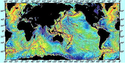
Seasat was the first U.S. satellite that, as an original intention, had as its primary mission, monitoring oceanic surface phenomena, such as sea state (surface wave parameters, including wavelength, period, and height), surface wind fields, internal waves, currents and eddies, and sea ice characteristics. The microwave systems on Seasat were described on page 8-6; on that same page is the remarkable map of fractures systems in the global ocean floor. Here we present a JPL image of worldwide generalized sea surface height derived from Seasat data:
Radar images from Seasat over land surfaces proved so invaluable that the impression may be that we subordinated the marine applications. Nevertheless, the system performed well as intended and we gleaned much information about the oceans during its 98 days of service in 1978, before an electrical short circuit disabled it.

Intersecting waves are strongly expressed in this Terra ASTER (sensor) image of waters in the Bay of Bengal east of India.
Many wave sets have wavelengths and amplitudes that are small compared to those in the open oceans, in part because of limited fetch (area over which the waves are generated by winds). These require high resolution imagery to detect. Here is a 4-meter resolution IKONOS blue band image of a lake in Mississippi in which the wave train has a northeast directionality:

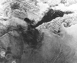
Surface wave expressions related to variations in bathymetric depths are evident in the right Seasat image (north to upper left), showing the Nantucket Shoals off Rhode Island. Nantucket Island is at the bottom left.

Internal waves, such as those shown in the Sulu Sea (Pacific Ocean), result when a subsurface layer of water with different density and temperature is moved by currents against the upper layer. No surface crests are formed but the motion produces an interference effect visible as dark bands.

Internal (subsurface) waves in shallow waters in the Gulf of California appear in the next Seasat image on the left (north is towards the lower right).
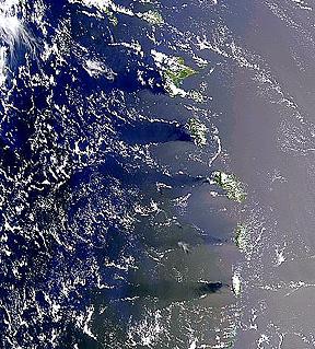
An interesting phenomenon known as “wake effect” is evident in this SeaWiFS (see next page) image of the Windward Islands in the eastern Caribbean. Prevailing winds from the east encounter topographic highs (mostly volcanic peaks) and are disrupted and slowed down. This leaves calmer surface winds, and much reduced wave heights, on the leeward side. Sun glint helps to emphasize the contrast.
We first described the TOPEX-Poseidon (T/P) mission, run by JPL, in page 8-7. We suggest you access this (outstanding tutorial) prepared by the TOPEX-Poseidon team, which explores the kinds of information that radar altimetry and scatterometry can acquire.
TOPEX-Poseidon uses two radar altimeters to measure distance from the satellite to the sea’s surface (to a precision of 4.3 cm). From such data, we derive global maps that show Dynamic Ocean Topography (rises [“hills”] and depressions [“valleys”]), Sea Surface Variability, Wave Heights, and Wind Speeds. A separate microwave radiometer on this mission determines Precipitable Water Vapor, which allows for corrections in the pulse transit time to improve distance accuracy.
` <>`__14-31: How would T/P determine wind speeds from the observables? **ANSWER**` <Sect14_answers.html#14-30>`__
The first TOPEX-Poseidon maps we examine show ocean topographic variations. Below is a plot of large-scale variations during September 1992 in ocean elevations relative to the Earth’s geoid. The data used to construct the map come from other sources, such as gravitational perturbations of satellite orbits. Note that, as much as 150 m (492 ft) of relief exist on the seas between the Atlantic Ocean (lower, green) and the western Pacific (higher, orange-red).
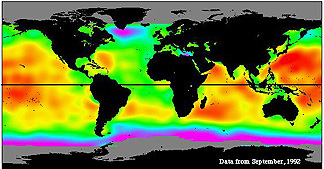
` <>`__14-32: Where are the oceans the highest? **ANSWER**
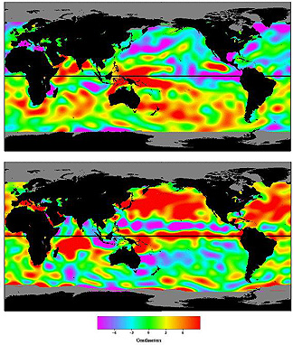
Seasonal differences do occur because of departures from the norms in height, as water expands or contracts in each hemisphere. The pair of maps below show Sea Surface Height (SSH) variationin the northern Fall (upper) and Spring (lower), in a plot centered on the Pacific Ocean. The differences in elevation lead to redistribution of water through thermally-induced currents.

TOPEX-Poseidon also has shed new light on the oceans tides. There has been an ongoing mystery as to balancing the energy provided by the Moon’s gravitational attraction, which produces the tides, and the dissipation of that energy. What was known is that much of the energy goes into setting up surficial ocean currents that carry water from higher areas to lower. Ocean heights measurements by T-P have now better fixed the areas of the seas that are higher and lower than mean sea level. This image shows a general pattern:
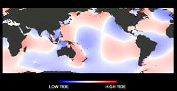
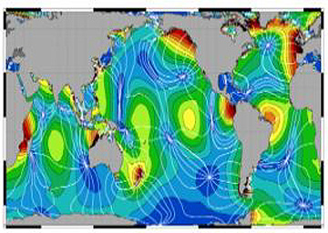
And this image shows more details, representing a data sets for six years of observations. The so-called tidal energy dissipation thus displayed is affected in part by variations in sea surface heights which establish gradients that cause water flow that influences tidal rises or falls (see page I-1b.

From this can be derived this broad outline of the current flow lines outward from the highs:
The shortfall of about 30% for the accounting of energy balance in tidal energy distribution has from the T-P observations now been explained by work done in changing ocean volume below the surface. The configuration of the sea floor contributes to this.
A follow-up to TOPEX-Poseidon, named JASON-1, is a component of the EOS program (see Section 16). Operated jointly by NASA JPL/CNES, this spacecrafts sensors include C and Ku band radar altimeters, a microwave radiometer, and a Doppler radar. Again, sea surface heights (SSH) are the main oceanographic phenomenon being measured; for Jason, differences in SSH as small as 4.1 cm can be determined.
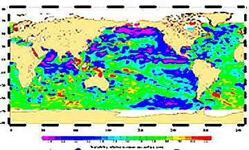
Data from Jason-1 are now being processed routinely by various government and private centers engaged in marine studies. This map of global tropical zones was produced by the Space Center at the Univesity of Texas-Austin.
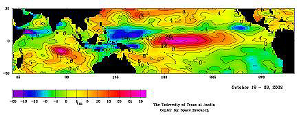
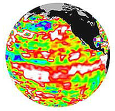
Just as has been done by Topex-Poseidon for the last 10 years, Jason-1 is gathering daily information on the buildup of hot waters that lead to the El Niño that forms every several years in the Pacific. Here is an October, 2002 Jason-1 map that shows the warming trend in the eastern Pacific - as the winter of 2002-03 ensues, unusual weather has indeed become common in the United States.
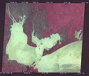
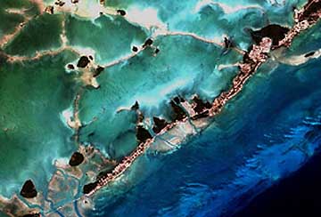
One aspect of oceanographic studies and management that has received considerable attention lately is the state of health of corals - the animals (polyps) that make the foundation of coral reefs which support a wide variety of biota. Various satellites are contributing to an organized monitoring program designed to gather long term data and to “flag” potential local to worldwide conditions that threaten coral populations. Landsat 7 is a mainstay of this effort. Here is a Landsat false color view of part of the Florida Keys (see also page 8-6) which illustrates the monitoring capabilities from satellites.
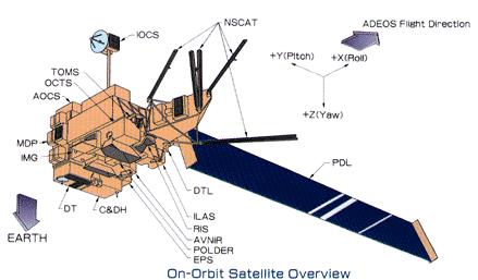
Turning again to the Japanese ADEOS (Midori), as expected it carries a Vis-NIR imager (called AVNIR). Here is an image of some of the island reefs in the Great Barrier Reef of northeast Australia.
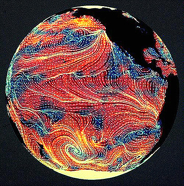
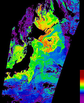
ADEOS also produced some interesting ocean color images, none more so than this view of the sea around Japan itself, here with the natural colors modified to the full range of blues through reds to emphasize currents and other water circulation patterns:
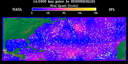
NSCAT was a microwave radar scatterometer that transmitted pulses at 13.995 GHz and measured their reflections (backscatter) from ocean ripples and other surfaces. Six antennas provided eight beams that extended over two wide bands. The returned signal is subjected to Doppler processing. In general, rougher seas correlate with greater wind speeds; in turn, rough seas increase backscatter. Operating at 50 km spatial resolution, the system distinguished and recorded 268,000 wind vectors, derived from wave-induced backscatter data.

Further processing allows imposition of pseudo-streamlines indicating wind direction, as shown here:

On July 19, 1999 NASA JPL launched QuickScat, a satellite whose prime sensor (SeaWinds) is a radar with 25 meter resolution. Its primary mission is to provide near-realtime measurements of surface roughness that translate into wind velocities. Below is a map of Hurricane Alley in low latitudes of the Atlantic, on which color shading indicative of wind speeds and vectors showing prevailing wind directions are plotted.
And here is a QuickScat SeaWinds map that includes an actual hurricane, Floyd, a destructive one that hit the southern U.S. in September, 1999; the immediate area of the hurricane appears as an expanded inset:
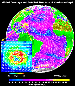
That localized area is shown in more detail in this SeaWinds map of wind flow in the Gulf of Mexico and the Atlantic during Hurricane Floyd on September 16, 1999:

NASA sponsored another SeaWinds radar scatterometer as an instrument package onboard ADEOS-2 (renamed Midori-2) launched on December 14, 2002 by the Japanese NASDA program. Primarily an ocean surface monitor, this sensor can identify sea ice and can, like its predecessors above, determine wind velocities. Here is the first returned data set acquired on January 28-29, 2003:
|SeaWinds January 2003 global data showing polar ice as gray and ocean wind speeds as low (blue) to high (red). |
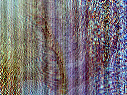
The Japanese have also launched several Marine Observation Satellites (MOS) that include their own scanning radiometer (MESSR), a Visible-Thermal instrument (VTIR), and a microwave unit (MSR). These sensors are operated over both land and sea. This MESSR image of the south-central coast of Japan, showing bays below the city of Nagoya, is typical.