Untitled
Contents
Remote Sensing Tutorial Introduction - Part 2 Page 1
This page is devoted to the study from space of the Earth’s gravity and what departures (anomalies) from a uniform gravitational field tell us about the distribution of mass (density variations) primarily in the outer region called the lithosphere. The coverage begins with a review of the real and mathematical shapes appropriate to the whole Earth. The Earth’s general figure (shape) approaches that of a pole-flattened ellipsoid. A mathematically-defined surface approximating the gravity equipotential is referred to as the geoid. Gravitational variations owing to topography, crustal structure, and rock type differences provide departures - anomalies - which can be measured from orbiting satellites. Information about these variations comes from analyzing the changes in orbital paths. Satellites have also been able to determine the variations in sea surface heights which tend to reproduce the variations in ocean floor topography. Radar and laser altimetry from these satellites can directly measure these height differences. Global geoid and topography maps have resulted from such investigations.
In geophysics, especially that applied branch dedicated to exploration for mineral/energy resources, there are three main fields or subdivisions: Magnetics, Gravity, and Seismology. The last finds limited opportunities from space but will be touched upon here as it applies to crustal dyanamics. Most of the subject matter on this page deals with gravity.
We assume that you have some familiarity (most likely from a physics course) with the basic notion of gravity. The fundamental law, proposed by Newton, is F = G (m:sub:1m2/r:sup:2) = ma, where the two m’s are masses (e.g., the Earth and you), the m without a subscript is the mass of any body at the surface or falling from above, r is the distance between the centers of masses m1 and m2, and G is the Universal Gravitational Constant (G = 6.6726…x 10-11 m3-kg:sup:-1-sec:sup:-2). We will not attempt much more consideration of the (physics) basics, but will start by describing some of the main ideas and terms associated with measuring gravity, gravity variations (anomalies), and techniques for obtaining data which can be reduced to a reference state (the ellipsoid) to compare with actual Earth conditions.
We begin by considering terrestrial gravity as it relates to the actual and the theoretical shapes or figure of the Earth - the subject matter of Geodesy.
Ideally, the Earth might have been a perfect sphere composed of a single substance, homogeneously distributed and with a uniform density throughout. A single value of gravity would prevail, determined by Newton’s equation. The actual Earth consists of three major zones concentric about its center (where all its mass is said to concentrate for purposes of calculating its gravity): a Core (solid Inner; a thick liquid Outer Core); a Mantle (somewhat variable in mass distribution and density); and a Lithosphere (made up part of the Upper Mantle and two types of crust - oceanic (more uniform in composition) and continental (variable in thickness and notably heterogeneous). For several reasons, the strength of gravity at the Earth’s real surface (the topographic surface) varies from place to place. These include the influence of different rock types (and densities), hot spot sources and mantle convection, and structural/topographic irregularities.
Gravity is usually measured in units of acceleration, as gals (or in mapping, as milligals) with a standard value (which has varied slightly as better measurments refine it) at 981.275 centimeters per second per second. (On the ground, the measurements are made either with a pendulum-based apparatus or, now more commonly, a gravimeter (weight on a spring).
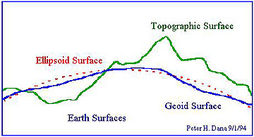
Ignoring the surficial irregularities for the moment, the Earth’s general shape departs slightly from a sphere. The Earth Ellipsoid is an oblate ellipsoid, with its average radius from center to equator (semi-major axis) being 6,378.16… km and center to pole (semi-minor axis) being 6,356.77… km; this amounts to a polar shortening of 1 part in 298.25. The ellipsoid, which actually doesn’t exist except for calculational purposes, would have a regular, smooth surface.
Departures from the ellipsoidal surface caused by differences in gravitational attraction caused by variations in density produce another reference (mathematically-computed, not actual) surface called the geoid. The geoid has been defined as “the (undulating) surface assumed by an undisturbed (perfectly calm) top of the sea, and visualized as continuing under the continents by water filling (hypothetical) small frictionless channels (canals).” It thus closely approximates the variations in heights of existing sea level and hypothetical extensions of the sea through the continents. Related to it is sealevel equipotential, a surface on which gravity is everywhere equal to its strength at mean sea level. The geoidal surface shows broad undulations related to underlying masses. This diagram may help to envision this:
Geoidal data can be derived from satellite measurements. This happens because satellites move up and down along their orbits as they are affected by the same gravitational forces that produce the geoidal surface. Here is a plot of changes in geoid height along a 70 km track as derived from data measured by the ERS-2 satellite (see below).

Over the years gravity measurements have led to both generalized and regional models of the geoid. Here is a colored representation of the coarse (10 ° by 10 °) geoidal surface in the standard 1984 World Geodetic System version:

In 1996, a more detailed and definitive Earth Geoidal Model, showing the global geopotential surface, was produce by the National Imagery and Mapping Agency, NASA Goddard, and the Ohio State and Texas Universities, using data from Topex-Poseidon, GPS, SLR, DORIS, and TDRSS. The improved version adds information from spherical harmonics coefficient analysis and newer free air anomaly corrections

At higher resolution, is the the geoidal surface for the United States and parts of Mexico and Canada:

Geoidal surfaces can be calculated for ocean surfaces as well. This is a plot (strong vertical exaggeration) of part of the Indian Ocean. The irregularities are partly due to ocean floor topography (see below).

As can be seen from the above illustrations, the geoid tends to be higher in the continents and (relatively) lower in the oceans.
Gravity measurements are usually referenced to the ellipsoid, or for some puposes to the geoid. Gravitational measurements on the ground, from ships, or from space after suitable data reductions will typically give rise to values that are higher (positive anomalies) or lower (negative anomalies than the gravitational potential assigned to the equipotential surface. Several “corrections” must be applied. For instance, for a gravimeter at an elevation above sea level, the free air correction adjusts the gravity reading to what it ought to be at mean sea level. A typical adjustment rate is 1 milligal per 3 meters (added if above sea level; subtracted if below). Another correction is made to compensate for the slight increase in gravity going poleward (this ranges from 978.04 at the equator to 983.2 cm/sec/sec at the pole, where the instrument would be closer to the center of mass). The Bouguer correction removes the effect of any topographic mass (such as mountains) lying above or below the ellipsoid. When all appropriate corrections are made, the observed gravity reading is compared to the predicted or calculated reading based on a geoidal distribution. Any difference is the Bouguer Anomaly which is largely due to solid earth masses in the crust, or deeper, owing to different rock types and rock densities.
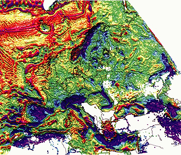
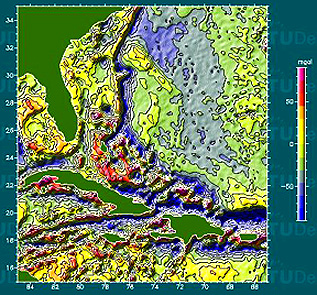
As indicated above, continental gravity surveys have made use of field instruments such as gravimeters. Much of the data have been collected for regions of interest in oil/gas exploration. Surveys can be made from low, slow flying aircraft or helicopters and make measurements with accelerometers and gradiometers. One difficulty is accurate location of the flight line; the development of the multiple satellite Global Positioning System (GPS) has improved the ability to track the flight lines with high accuracy. The data after acquisition must be processed to make the appropriate corrections described above. Ground/aircraft gravity anomalies made from different surveys can be integrated into regional maps or even at the scale of continents. Below is a gravitational anomaly map (Bouguer on land; Free Air anomalies over water) (positive anomalies in red, with maximum at +75 milligals; negative in blue, minimum at - 75 mgal) of most of Europe, the Mediterranean, and the North Atlantic (the outlines of countries in black are there but hard to see; to get your bearings, the dark blue area near the top is Norway; a similar color below center is the Po Valley south of the Alps:
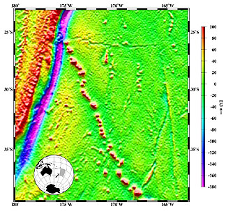
A gravity map of Australia (at lower mgal resolution) made by air/ground surveys and its surrounding oceanic floor as made with satellite data is a clear example of how both near-surface and spaceborne gravity-measuring systems can be combined to make a gravity map:

Now, on to the role that satellites play in determining Earth’s gravitational field and anomalies. Two figures indicate how well gravsats (a term for satellites used to obtain information on gravity, introduced here for to foster brevity; do not confuse it, with the name of a British Company, Gravsat, that commercially supplies satellite data) can duplicate or approximate gravity data acquired on the ground and by air. Both are in units of mgals: the top is the tracing of gravitational changes measured along a satellite track crossing the South China Sea as compared with readings from a shipborne gravimeter following the same line; the lower figure shows a gravitational anomaly map of an oceanic area on the left and a map obtained by using limited field data from a marine survey.


As a general statement: the prime use and successes of gravity satellites have been in surveying the topography of oceans and other large bodies of water. Because of their high rates of orbital velocity and other complications, satellites do not normally carry accelerometers (which have low response times) to measure direct changes in gravitational attraction along their orbital tracks. Instead, gravity variations can be calculated from changes in the position (shifts in orbital height) of a satellite as it orbits - these are caused by the varying force of gravity from both the transient nadir points and surrounding areas near the path trace. Tracking of radio signals (using Doppler shifts in frequency) from the satellite help to determine these variations. A more direct way is to follow the satellite’s path or locate its position with a technique called satellite laser ranging (SLR). The other major approach is to measure, from the satellite itself, the changing heights of the surface (using that of sea level with reference to the geoid) by either radar altimetry or laser altimetry.
The principle behind measuring the changes in sea surface elevations (which can vary as much as 160 meters over the Earth’s oceans) is evident in this diagram:

The presence of this extra mass above the sea floor is to cause of deviation of gravitational attraction forces such that water about the seamount bunches up into a rise or mound. If instead there were a depression (e.g., oceanic trench) on the floor, the drop in gravity owing to absence of material (mass) in the trench space would cause a depression of the water at the surface. In other words, the sea surface roughly mirrors (reproduces) the topographic variations of the sea floor. Simply by measuring the distance between a satellite sending a signal (that returns) and the water surface, an anomaly N is created, as shown in this next figure (where N = h* - h; h* is the distance to the calculated geoid for the area and h is the signal path distance of the surface bulge to the satellite).

This approach was first tested by an experiment on Skylab. Proof of concept was then dramatically demonstrated by the radar altimeter on Seasat (see page 8-6). Altimetry data from this mission led to the now famous general map of the world’s ocean floors (bottom of p. 8-6), with their structural patterns reflected in their topography, was constructed by marine geophysicists. Radar altimeters now operate (or have earlier) from a host of satellites including Seasat, Geosat, Topex-Poseidon, ERS-1 and -2, Geos3; new systems will be onboard Envisat and JASON-1 to be launched later. Radar interferometry is also used for sea state studies(see page 8-7). Laser altimeters (which send out pulses of coherent light) are increasingly being deployed on aircraft and have flown on two Space Shuttle missions and will be on the GLAS (Geoscience Laser Altimeter System) now in planning. Lasers also were on a Mars spacecraft. The application of lasers from moving platforms are summarized in this diagram developed for the Shuttle Laser Altimeter (SLA) experiments:

On the remainder of this page we will give some examples of ocean floor gravity anomalies and a topography interpretation that have resulted from satellite altimetry.
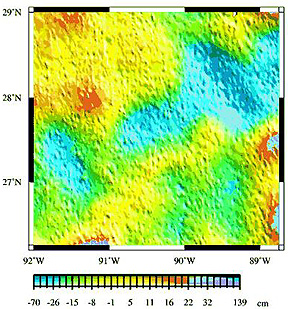
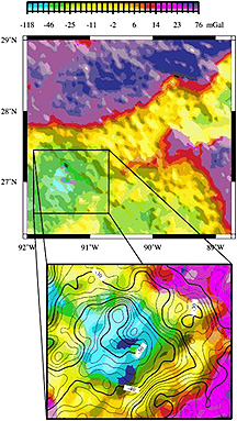
First are two maps of part of the Gulf of Mexico made from ERS-1 and Geosat data combined that are part of the study of that region in the Getech project (University of Leeds). The map on the left is a geoidal base showing mean sea level variations. On the right is the same area now converted to gravitational variations (in mgals) that indicate the influence of ocean floor configuration.
To the east is the ocean off the Florida coast, with determinations of gravity anomalies extracted from ERS-1 altimeter data.
Here is a gravity anomaly map of a region in the southwest Pacific in which one of the major ocean trenches (Tonga-Kermadee, on the left) is easily recognized, as are a series of small ocean floor volcanoes making up seamounts. This map emphasizes the fact that the gravitational variations tend to define the actual topography of the crust at its interface with the ocean.
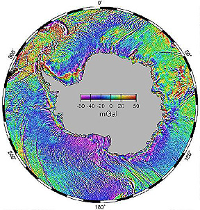
Now, examine this gravity map of the Southern Oceans around Antarctica.
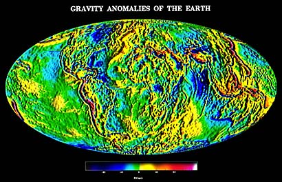
Various maps of global gravity variations have been constructed for both continents and ocean floors combined of which this is typical:
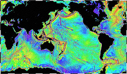
Likewise, maps showing just the sea floor gravity anomalies have been published:
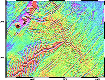
Maps of the actual ocean bottom surface (its topography) resemble the gravity maps closely since they commonly use the same color scheme (blue for low; red for high). These maps are nearly identical to bathymetric maps (those that show the thickness of the ocean water cover - depths). Here is a topographic map of the ridge and transform fault system in part of the western Indian Ocean:
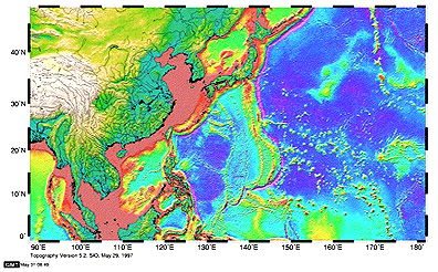
This is part of a global land and ocean topography map produced by Smith and Sandwell; it covers a 45 by 45° area that includes part of China and Southeast Asia and marine topography from north of Japan to Indonesia eastward into the western Pacific.
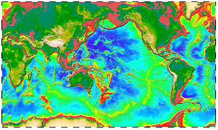
The full Smith and Sandwell first order topographic map (1995) for the whole world is reproduced here:
The latest geophysical-gravity satellite is GRACE (Gravity Recovery and Climate Experiment), launched on March 17, 2002. GRACE is actually a pair of satellites in the same orbit at 500 km but 220 km apart (formation flying). The precise location of each satellite is constantly determined by their radio interaction with Global Positioning Satellites (GPS). Each GRACE satellite uses microwave signals to determine very precisely the vertical distance between spacecraft and points on the ocean surface (and land as well) to get a sea surface height that is 103 times more accurate than previous systems. This yields a much more detailed picture of the geoid, or mean gravity field. This first global image shows a remarkable feature:
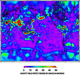
That feature is the excellent definition of subduction zones at converging plate boundaries. These are the patterns that are displayed in reds. Note especially the Aleutian chain, the Indonesian chain, and the Himalayan-Indian boundary.
In July 2003, the GRACE team released the most accurate (by a factor better than 10x) yet gravity map of the entire world. The geoid represented shows variations that indicate the geoidal surface (its real differences in height after currents, wind, and tide effects are removed that are just under 200 m (650 ft). This represents the ability now to show variations at the centimeter level.

GRACE will continue to acquire high sensitivity data for up to 5 years; from the data sets gravity profiles will be constructed.Global gravity map made from GRACE microwave measurements