Sensor Technology
Contents
Remote Sensing Tutorial Introduction - Part 2 Page 5a
In the first 5 pages of this Introduction, emphasis has been placed on the nature and properties of the electromagnetic radiation that is the information carrier about materials, objects and features which are the targets of interest in remote sensing. But to gather and process that information, devices called sensors are needed to detect and measure the radiation. This page looks at the basic principles involved in sensor design and development. A classification presented here indicates the variety of sensors available to “do the job”. Discussion of film camera systems and radar is deferred to other Sections. This page concentrates on scanning spectroradiometers, a class of instruments that is the “workhorse” in this stable of remote sensors.
Sensor Technology
So far, we have considered mainly the nature and characteristics of EM radiation in terms of sources and behavior when interacting with materials and objects. It was stated that the bulk of the radiation sensed is either reflected or emitted from the target, generally through air until it is monitored by a sensor. The subject of what sensors consist of and how they perform (operate) is important and wide ranging. It is also far too involved to merit an extended treatment in this Tutorial. However, a synopsis of some of the basics is warranted on this page. A comprehensive overall review of Sensor Technology, developed by the Japanese Association of Remote Sensing, is found on the Internet at this mirror site. Some useful links to sensors and their applications is included in this NASA site.
Most remote sensing instruments (sensors) are designed to measure photons. The fundamental principle underlying sensor operation centers on what happens in a critical component - the detector. This is the concept of the photoelectric effect (for which Albert Einstein, who first explained it in detail, won his Nobel Prize [not for Relativity which was a much greater achievement]; his discovery was, however, a key step in the development of quantum physics). This, simply stated, says that there will be an emission of negative particles (electrons) when a negatively charged plate of some appropriate light-sensitive material is subjected to a beam of photons. The electrons can then be made to flow from the plate, collected, and counted as a signal. A key point: The magnitude of the electric current produced (number of photoelectrons per unit time) is directly proportional to the light intensity. Thus, changes in the electric current can be used to measure changes in the photons (numbers; intensity) that strike the plate (detector) during a given time interval. The kinetic energy of the released photoelectrons varies with frequency (or wavelength) of the impinging radiation. But, different materials undergo photoelectric effect release of electrons over different wavelength intervals; each has a threshold wavelength at which the phenomenon begins and a longer wavelength at which it ceases.
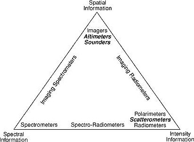
Now, with this principle established as the basis for the operation of most remote sensors, let us summarize several main ideas as to sensor types (classification) in these two diagrams:
The first is a functional treatment of several classes of sensors, plotted as a triangle diagram, in which the corner members are determined by the principal parameter measured: Spectral; Spatial; Intensity.
The second covers a wider array of sensor types:

From this imposing list, we shall concentrate the discussion on optical-mechanical-electronic radiometers and scanners, leaving the subjects of camera-film systems and active radar for consideration elsewhere in the Tutorial and holding the description of thermal systems to a minimum (see Section 9 for further treatment). The top group comprises mainly the geophysical sensors we considered earlier in this Section.
The two broadest classes of sensors are Passive (energy leading to radiation received comes from an external source, e.g., the Sun) and Active (energy generated from within the sensor system, beamed outward, and the fraction returned is measured). Sensors can be non-imaging (measures the radiation received from all points in the sensed target, integrates this, and reports the result as an electrical signal strength or some other quantitative attribute, such as radiance) or imaging (the electrons released are used to excite or ionize a substance like silver (Ag) in film or to drive an image producing device like a TV or computer monitor or a cathode ray tube or oscilloscope or a battery of electronic detectors (see further down this page for a discussion of detector types); since the radiation is related to specific points in the target, the end result is an image [picture] or a raster display [as in:the parallel lines {horizontal} on a TV screen).
Radiometer is a general term for any instrument that quantitatively measures the EM radiation in some interval of the EM spectrum. When the radiation is light from the narrow spectral band including the visible, the term photometer can be substituted. If the sensor includes a component, such as a prism or diffraction grating, that can break radiation extending over a part of the spectrum into discrete wavelengths and disperse (or separate) them at different angles to detectors, it is called a spectrometer. One type of spectrometer (used in the laboratory for chemical analysis) passes multiwavelength radiation through a slit onto a dispersing medium which reproduces the slit as lines at various spacings on a film plate. The term spectroradiometer tends to imply that the dispersed radiation is in bands rather than discrete wavelengths. Most air/space sensors are spectroradiometers.
Sensors that instantaneously measure radiation coming from the entire scene at once are called framing systems. The eye, a photo camera, and a TV vidicon belong to this group. The size of the scene that is framed is determined by the apertures and optics in the system that define the field of view, or FOV. If the scene is sensed point by point (equivalent to small areas within the scene) along successive lines over a finite time, this mode of measurement makes up a scanning system. Most non-camera sensors operating from moving platforms image the scene by scanning.
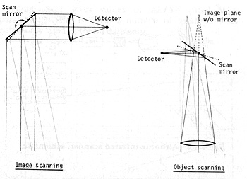
Moving further down the classification tree, the optical setup for imaging sensors can be image plane or optical plane focused (depending on where the photon rays are converged by a lens), as shown in this illustration.
Another attribute in this classification is whether the sensor operates in a non-scanning or a scanning mode. This is a rather tricky pair of terms that can have several meanings in that scanning implies motion across the scene over a time interval and non-scanning refers to holding the sensor fixed on the scene or target of interest as it is sensed in a very brief moment. A film camera held rigidly in the hand is a non-scanning device that captures light almost instantaneous when the shutter is opened, then closed. But when the camera and/or the target moves, as with a movie camera, it in a sense is performing scanning as such. Now, the target can be static (not moving) but the sensor sweeps across the sensed scene, which can be scanning in that the sensor is designed for its detector(s) to move systematically in a progressive sweep even as they also advance across the target. This is the case for the scanner you may have tied into your computer; here its flatbed platform (the casing and glass surface on which a picture is placed) also stays put; scanning can also be carried out by put a picture or paper document on a rotating drum (two motions: circular and progressive shift in the direction of the drum’s axis) in which the scanning illumination is a fixed beam. Or, two other related examples: A TV camera containing a vidicon in which light hitting that photon-sensitive surface produces electrons that are removed in succession (lines per inch is a measure of the TV’s performance) can either stay fixed or can swivel to sweep over a scene (itself a spatial scanning operation) and can scan in time as it continues to monitor the scene. A digital camera contains an X-Y array of detectors that are discharged of their photon-induced electrons in a continuous succession that translate into a signal of varying voltage. The discharge occurs by scanning the detectors systematically. That camera itself can remain fixed or can move. The gist of all this (to some extent obvious) is that the term scanning can be applied both to movement of the entire sensor and, in its more common meaning, to the process by which one or more components in the detection system either move the light gathering, scene viewing apparatus or the light or radiation detectors are read one by one to produce the signal. Two broad categories of most scanners are defined by the terms “optical-mechanical” and “optical-electronic”, distinguished by the former containing an essential mechanical component (e.g., a moving mirror) that participates in scanning the scene and the latter by having the sensed radiation move directly through the optics onto the linear or array detectors.
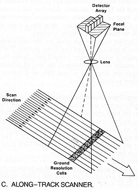
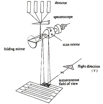
Another attribute of remote sensors, not shown in the classification, relates to the modes in which those that follow some forward-moving track (referred to as the orbit or flight path) gather their data. In doing so, they are said to monitor the path over an area out to the sides of the path; this is known as the swath width. The width is determined by that part of the scene encompassed by the telescope’s full angular FOV which actually is sensed by a detector array - this is normally narrower than the entire scene’s width from which light is admitted through the external aperture (usually, a telescope). The principal modes are diagrammed in these two figures:
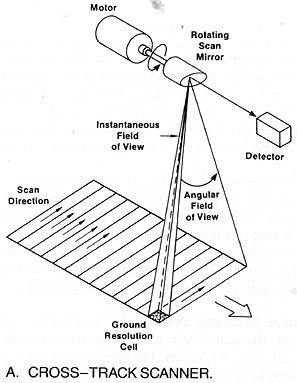
The Cross Track mode normally uses an rotating (spinning) or oscillating mirror (making the sensor an optical-mechanical device) to sweep the scene along a line traversing the ground that is very long (kilometers; miles) but also very narrow (meters; yards), or more commonly a series of adjacent lines. This is sometimes referred to as the whiskbroom mode from the vision of sweeping a table side to side by a small handheld broom.) A general scheme of a typical Cross-Track Scanner is shown below. The essential components of this instrument (most are shared with Along Track systems) are 1) a light gathering telescope that defines the scene dimensions at any moment (not shown); 2) appropriate optics (e.g., lens) within the light path train; 3) a mirror (on aircraft scanners this may completely rotate; on spacecraft scanners this usually oscillates over small angles); 4) a device (spectroscope; spectral diffrqction grating; band filters) to break the incoming radiation into spectral intervals; 5) a means to direct the light so dispersed onto a battery or bank of detectors; 6) an electronic means to sample the photo-electric effect at each detector and to then reset to to a base state to receive the next incoming light packet, resulting in a signal that relates to changes in light values coming from the ground or target; and 7) a recording component that either reads the signal as an analog (displayable as an intensity-varying plot (curve) over time or converts the signal to digital numbers. A scanner can also have a chopper which is a moving slit or opening that as it rotates alternately allows the signal to pass to the detectors or interrupts the signal (area of no opening) and commonly redirects it to a reference detector for calibration of the instrument response.
Each line is subdivided into a sequence of individual spatial elements that represent a corresponding square, rectangular, or circular area (ground resolution cell) on the scene surface being imaged (or in, if the target to be sensed is the 3-dimensional atmosphere). Thus, along any line is an array of contiguous cells from each of which emanates radiation. The cells are sensed one after another along the line. In the sensor, each cell is associated with a pixel (picture element) that is tied to a microelectronic detector; each pixel is characterized for a brief time by some single value of radiation (e.g., reflectance) converted by the photoelectric effect into electrons.
The areal coverage of the pixel (that is, the ground cell area it corresponds to) is determined by instantaneous field of view (IFOV) of the sensor system. The IFOV is defined as the solid angle extending from a detector to the area on the ground it measures at any instant (see above illustration). IFOV is a function of the optics of the sensor, the sampling rate of the signal, the dimensions of any optical guides (such as optical fibers), the size of the detector, and the altitude above the target or scene. The electrons are removed successively, pixel by pixel, to form the varying signal that defines the spatial variation of radiance from the progressively sampled scene. The image is then built up from these variations - each assigned to its pixel as a discrete value called the DN (a digital number, made by converting the analog signal to digital values of whole numbers over a finite range [for example, the Landsat system range is 28, which spreads from 0 to 255]). Using these DN values, a “picture” of the scene is recreated on film (photo) or on a monitor (image) by converting a two dimensional array of pixels, pixel by pixel and line by line along the direction of forward motion of the sensor (on a platform such as an aircraft or spacecraft) into gray levels in increments determined by the DN range.
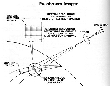
The Along Track mode does not have a mirror looking off at varying angles. Instead there is a line of small sensitive detectors stacked side by side, each having some tiny dimension on its plate surface; these may number several thousand. Each detector is a charge-coupled device (CCD), as described in more detail below on this page. In this mode, the pixels that will eventually make up the image correspond to these individual detectors in the line array. As the platform advances along the track, at any given moment radiation from each ground cell area along the ground line is received simultaneously at the sensor and the collection of photons from every cell impinges in the proper geometric relation to its ground position on every individual detector in the linear array equivalent to that position. The signal is removed from each detector in succession from the array in a very short time (milliseconds), the detectors are reset to a null state, and are then exposed to new radiation from the next line on the ground that has been reached by the sensor’s forward motion. This type of scanning is also referred to as pushbroom scanning (from the mental image of cleaning a floor with a wide broom through successive forward sweeps). As signal sampling improves, the possibility of sets of linear arrays, leading to area arrays, all being sampled at once will increase the equivalent area of ground coverage.
On the remainder of this page, we will concentrate on scanning spectroradiometers. The common components of a sensor system are shown in this table (not all need be present in a given sensor, but most are essential):

This next figure is a diagrammatic model of an electro-optical sensor that does not contain the means to break the incoming radiation into spectral components (essentially, this is a panchromatic system in which the filter admits a broad range of wavelengths). The diagram contains some of the elements found in the Return Beam Vidicon (TV-like) on the first two Landsats. Below it is a simplified cutaway diagram of the Landsat Multispectral Scanner (MSS) which through what is here called a shutter wheel or mount, containing filters each passing a limited range of wavelength, the spectral aspect to the image scanning system is added, i.e., produces discrete spectral bands:
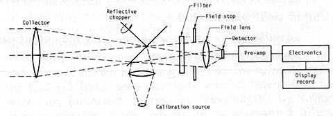
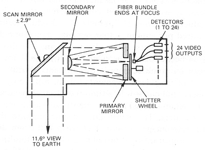
The front end of a sensor is normally a telescopic system (in the image denoted by the label 11.6°) to gather and direct the radiation onto a mirror or lens. The mirror rocks or oscillates back and forth rapidly over a limited angular range (the 2.9 ° to each side). In this setup, the scene is imaged only on one swing, say forward, and not scanned on the opposing or reverse swing; or, active scanning can occur on both swings. Some sensors allow the mirror to be pointed off to the side at specific fixed angles to capture scenes adjacent to the vertical mode ground track (SPOT is an example). In a pushbroom scanner, a chopper may be in the optic train near this point. It is a mechanical device to interrupt the signal either to modulate or synchronize it or, commonly, to allow a very brief blockage of the incoming radiation while the system looks at an onboard reference source of radiation of steady, known wavelength(s) and intensity in order to calibrate the final signals tied to the target. Other mirrors or lenses may be placed in the train to further redirect or focus the radiation.
The radiation - normally visible and/or Near and Short Wave IR, and/or thermal emissive in nature - must then be broken into its spectral elements, into broad to narrow bands. The width in wavelength units of a band or channel is defined by the instrument’s spectral resolution (see top of page 13-5). Prisms and diffraction gratings are one way to break selected parts of the EM spectrum into intervals; filters are another. In the above cutaway diagram of the MSS the filters are located on the shutter wheel. The first two spread the radiation at specific angles and need to have detectors placed where each wavelength-dependent angle directs the radiation. Or. for filter setups, the spectrally-sampled radiation is carried along optical fibers to dedicated detectors. Absorption filters pass only a limited range of radiation wavelengths, absorbing radiation outside this range. They may be either broad or narrow bandpass filters. This is a graph of a typical bandpass filter:

These filters may be high bandpass (selectively removes shorter wavelengths) or low bandpass (absorbs longer wavelengths). Interference filters work by reflecting unwanted wavelengths and transmitting others in a specific interval. A common type of filter used in general optics and on many scanning spectroradiometers is the dichroic filter.This uses an optical glass substrate over which are deposited (in a vacuum setup) from 20 to 50 thin (typically, 0.001 mm thick) layers of a special refractive index dielectric material (or materials in certain combinations) that selectively transmits a specific range or band of wavelengths. Absorption is nearly zero. These can be either additive or subtractive color filters when operating in the visible range.
The next step is to get the spectrally separated radiation to appropriate detectors. This can be done through lenses or by detector positioning or, in the case of the MSS and other sensors, by channeling radiation in specific ranges to fiber optics bundles that carry the focused radiation to an array of individual detectors. For the MSS, this involves 6 fiber optics leads for the six lines scanned simultaneously to 6 detectors for each of the four spectral bands, or a total of 24 detectors in all.
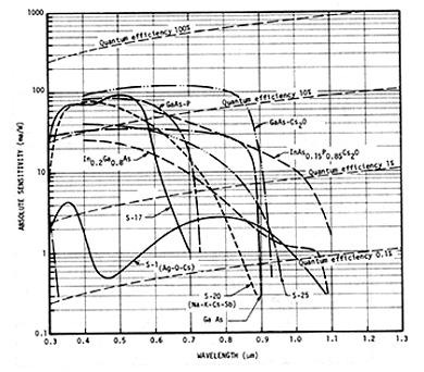
In the early days of remote sensing, photomultipliers served as detectors. Most detectors today are made of solid-state semiconductor metals or alloys. A semiconductor has a conductivity intermediate between a metal and an insulator. Under certain conditions, such as the interaction with photons, electrons in the semiconductor are excited and moved from a filled energy level (in the electron orbital configuration around an atomic nucleus) to another level called the conduction band which is deficient in electrons in the unexited state. The resistance to flow varies inversely with the number of incident photons. The process is best understood by quantum theory. Different materials respond to different wavelengths (actually, to photon energy levels) and are thus spectrally selective.
In the visible light range, silicon metal and PbO are common detector materials. Silicon photodiodes are used in this range. Photoconductor material in the Near-Ir includes PbS (lead sulphide) and InAs (indium-arsenic). In the Mid-IR (3-6 µm), InSb (indium-stibnium) is responsive.The most common detector material for the 8-14 µm range is Hg-Cd-Te (mercury-cadmium-tellurium); when operating it is necessary to cool the detectors to near zero Kelvin (using Dewars coolers) to optimize the efficiency of electron release. Other detector materials are also used and perform under specific conditions. This next diagram gives some idea of the variability of semiconductor detectivity over operating wavelength ranges.
Other detector systems, less commonly used in remote sensing function in different ways. The list includes photoemissive, photdiode, photovoltage, and thermal (absorption of radiation) detectors. The most important now are CCDs, or Charge-Coupled-Detectors, that are explained in the next paragraph. This approach to sensing EM radiation was developed in the 1970s, which led to the Pushbroom Scanner, which uses charge-coupled devices (CCDs) as the detector. This diagram may help to better grasp the description of CCDs in the next paragraph:
A CCD is an extremely small silicon chip, which is light-sensitive. When photons strike a CCD, electronic charges develop whose magnitudes are proportional to the intensity of the impinging radiation during a short time interval (exposure time). From 3,000 to more than 10,000 detector elements (the CCDs) can occupy a linear space less than 15 cm in length. The number of elements per unit length, along with the optics, determine the spatial resolution of the instrument. Using integrated circuits each linear array is sampled very rapidly in sequence, producing an electrical signal that varies with the radiation striking the array. This changing signal recording goes through a processor to a recorder, and finally, is used to drive an electro-optical device to make a black and white image, similar to MSS or TM signals. After the instrument samples the almost instantaneous signal, the array discharges electronically fast enough to allow the next incoming radiation to be detected independently. A linear (one-dimensional) array acting as the detecting sensor advances with the spacecraft’s orbital motion, producing successive lines of image data (analogous to the forward sweep of a pushbroom). Using filters to select wavelength intervals, each associated with a CCD array, we get multiband sensing. The one disadvantage of current CCD systems is their limitation to visible and near IR (VNIR) intervals of the EM spectrum. (CCDs are also the basis for two-dimensional arrays - a series of linear CCDs stacked in parallel to extend over an area; these are used in the now popular digital cameras and are the sensor detectors commonly employed in telescopes of recent vintage.)
Once a scanner or CCD signal has been generated at the detector site, it needs to be carried through the electronic processing system whose output is the signal used to make images or be analyzed (commonly as DN variations) by computer programs. Pre-amplification may be the first stage. Onboard digitizing is commonly applied to the signal and to the reference radiation source used in calibration. The final output is then sent to a ground receiving station, either by direct readout (line of sight) or through a satellite relay system like TDRSS (Tracking and Relay Satellite System; geosynchronous communications satellites). Another option is to record the signals on a tape recorder and play back the signals when the satellite can directly transmit to a receiving station (this was used on many of the earlier satellites, including Landsat [ERTS], both is now almost obsolete because of the much improved satellite communications network).
The subject of sensor performance is beyond the scope of this page. Three common measures will be mentioned: 1) S/N (signal to noise ratio; the noise can come from internal electronic components or the detectors themselves); 2) NEΔP and NEΔT, the Noise Equivalent Power (for reflectances) and 3) Noise Equivalent Temperature (for thermal emission), which relate to conditions between two adjacent detectors that affect their corresponding adjacent pixels.
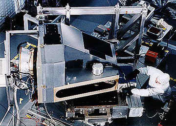
To tie the above theory to real systems, we show a photo of the MODIS sensor that now functioning well on the Terra spacecraft launched in late 1999 and Aqua two years later.
Finally, we need to consider one more vital aspect of sensor function and performance, namely the subject of spatial resolution. This concept is reviewed on page 10-3 as regards photographic systems and photogrammetry; check out that page at any time during these paragraphs. Here, we will attempt a generally non-technical overview of resolution.
Most of us have a strong intuitive feeling for the meaning of spatial resolution. Think of this experiential example. Suppose you are looking at a forested hillside some considerable distance away. What you see is the presence of the continuous forest but a great distance you do not see individual trees. As you go closer, eventually the trees, which may differ in size, shape, and species, become distinct as individuals. They have thus been resolved. As you draw much nearer, you start to see individual leaves. This means that the main components of an individual entity are now discernible and thus that category is being resolved. You can carry this ever further, through leaf macro-structure, then recognition of cells, and in principle with higher resolutions the individual constituent atoms and finally subatomic components. This last step is the highest resolution (related to the smallest sizes) achievable by instruments or sensors. All of these levels represent the “ability to recognize and separate features of specific sizes”. If you are looking at the scene from space, you might not be able to sense the presence of trees as discrete features because now the resolution is lower; from a very great distance the presence of a hill or mountain itself may not be detectable - its diagnostic features not being resolved.
The common sense definition of spatial resolution is often simply stated as the smallest size of an object that can be picked out from its surrounding objects or features. This separation from neighbors or background may or may not be sufficient to identify the object. Compare these ideas to the definition of three terms which have been extracted from the Glossary of Appendix D of this Tutorial:
resolution-Ability to separate closely spaced objects on an image or photograph. Resolution is commonly expressed as the most closely spaced line-pairs per unit distance that can be distinguished. Also called spatial resolution.
resolution target-Series of regularly spaced alternating light and dark bars used to evaluate the resolution of images or photographs.
resolving power-A measure of the ability of individual components. and of remote sensing systems, to separate closely spaced targets.
These three terms are defined as they apply to photographic systems (page 10-3 again). But resolution-related terms are also appropriate to electro-optical systems, standard optical devices, and even the human eye. The subject of resolution is more extensive and complicated than suggested from the above statements. Lets explore the ideas in more detail. The first fundamental notion is to differentiate resolution from resolving power. The former refers to the elements, features or objects in the target, that is the scene being sensed from a distance; the latter concerns the ability of the sensor, be it electronic or film or the eye, to separate the smallest features in the target that are the objects being sensed.
To help in the visualization of effective (i.e., maximum achieved) spatial resolution, lets work with a target that contains the objects that will be listed and lets use the human eye as the sensor, making you part of the resolving process, since this is the easiest notion involved in the experience. (A suggestion: Review the description of the eye’s functionality given in the answer to question I-1 [page I-1] in this Section.)
Start with a target that contains rows and columns of red squares each bounded by a thin black line place in contact with each other. The squares have some size determined by the black outlines. At a certain distance where you can see the whole target, it appears a uniform red. Walk closer and closer - at some distance point you begin to see the black contrasting lines. You have thus begun to resolve the target in that you can now state that there are squares of a certain size and these appear as individuals. Now decrease the black line spacing, making each square (or resolution cell) smaller. You must move closer to resolve the smaller squares. Or you must have improved eyesight (the rods and cones in the eye determine resolution; their sizes define the eye’s resolution; if some are damaged that resolution decreases).
Now modify the experiment by replacing every other square with a green version but keeping the squares in contact. At considerable distance neither the red nor green individuals can be specifically discerned as to color and shape. They blend, giving they eye (and brain processor) the impression of “yellowness” of the target (the effects of color combinations are treated also in Section 10). But as you approach, you start to see the two colors of squares as individuals. This distance at which the color pairs start to resolve is greater than the case above in which thin black lines form the boundary. Thus, for a given size, color contrast (or tonal contrast, as between black and white or shades of gray) becomes important in determining the onset of effective resolution. Variations of our experiment would be to change the squares to circles in regular alignments and have the spaces between the packed circles consist of non-red background, or draw the squares apart opening up a different background. Again, for a given size the distances at which individuals can first be discerned vary with these changing conditions. Still another modification would be to change the sizes and/or shapes of the individuals to be resolved; this would lead to other distances. One can talk now in terms of the smallest individual(s) in a collection of varying size/shape/color objects that become visibly separable - hence resolved.
Three variables control the achieved spatial resolution: 1) the nature of the target features as just specified, the most important being size; 2) the distance between the target and the sensing device; and 3) some inherent properties of the sensor embodied in the term resolving power. For this last variable, in the eye the primary factor is the sizes and arrangements of the rods and cones in the retina; in photographic film this is determined in part by the size of the AgCl grains or specks of color chemicals in the emulsion formed after film exposure and subsequent, although other properties of the camera/film system enter in as well.
For the types of sensors discussed on this page, there are several variable or factors that specify the maximum (highest) resolution obtainable. Obviously, first is the spatial and spectral characteristics of the target scene features being sensed, including the smallest objects who presence and identities are being sought. Next, of course, is the distance between target and sensor. For sensors in aircraft or spacecraft the interfering aspects of the atmosphere can degrade resolution. The speed of the platform, be it a balloon, an aircraft, an unmanned satellite, or a human observer in a shuttle or space station, is relevant in that it determines the “dwell time” available to the sensor’s detectors on the individual features from which the photo signals emanate.
Most targets have some kind of limiting area to be sensed that is determined by the geometric configuration of the sensor system being used. This is implied by the above-mentioned Field of View, outside of which nothing is “visible” at any moment. Commonly, this FOV is related to a telescope or circular tube that admits only light from the target at that particular moment. The optics in the telescope are important to the resolving power of the instrument; Magnification is one factor, as a lens system that increases magnifying capability also improves resolution. The spectral distribution of the incoming photons also plays a role. But, for sensors like those on Landsat or SPOT (described later in this Introduction and in other Sections), mechanical and/or electronic functions of the signal collection and detector components become the critical factors in obtaining improved resolution. This resolution is also equivalent to the pixel size. (The detectors themselves influence resolution by their inherent Signal to Noise (S/N) capability; this can vary in terms of spectral wavelengths). For an optical-mechanical scanner, the oscillation or rotation rate and arrangement of the scanning mirror motion will influence the Instantaneous Field of View IFOV) which is one of three factors that closely control the final resolution (pixel size) achieved. The second factor is related to the Size (dimensions) of an optical aperture that admits the light from an area on the mirror that corresponds to the segment of the target being sensed. For the Landsat MSS, as an example, the witdth of ground being scanned across-track is 480 m; the admitting and focusing optics break the width into 6 parallel scan lines that are directed to 6 detectors which account for the 80 meters (more exacting, 79 m) that form one pair of sides of a pixel. The third factor, which controls the cross-track boundary dimension of each pixel, is Sampling Rate of the continuous signal beam of radiation (light) sent by the mirror (usually through filters) to the detector array. For the Landsat MSS, this requires that all radiation received during the cross-track sweep along each scan line that fits into the IFOV (sampling element or pixel) be collected after every 10 microseconds of mirror advance by sampling each pixel independently in a very short time by electronic discharge of the detector. This sampling is done sequentially for the succession of pixels in the line. In 10 microseconds, the mirror’s advance is equivalent to sweeping 80 m forward on the ground; its cutoff to form the instantaneous signal contained in the pixel thus establishes the other two sides of the pixel (perpendicular to the sweep direction). In the first MSS, the dimensions thus imposed are equivalent to 79 by 57 meters, owing to the nature of the sampling process. Some of the ideas in the above paragraph, which may still seem tenuous to you at the moment, may be more comprehensible after reading page 16 of this Introduction which describes in detail the Landsat Multispectral Scanner. That page explains this 79 x 57 pixel geometry.
The preceding is a complicated concept in electronics that has only been mentioned broadly here; suffice to say that the signal must be subdividible into discrete packets that can be recorded as individual records of the amount and spectral nature of radiation from the surface target within the sensed IFOV - these become the pixels that can be digitized in DNs which in turn will be the fundamental “parcels” of information used to create images or otherwise provide data elements used to analyze and interpret the spatial and spectral entities in the target (which in a simple photograph stays put, but if imaged by a movie camera will produce a strip of successive images along the line of movement that convey a sense of the sequential motion of objects moving in time within the filmed scene or moving in location and time as the camera progresses along a line of flight, as is the case for flying or orbiting sensors).
The situation is somewhat different for sensors whose detectors are Charge-Coupled-Devices (CCDs). The relevant resolution determinants depend on the size of each fixed detector which in turn governs the sampling rate. That rate must be in “sync” with the ability to discharge each detector in sequence fast enough to produce an uninterrupted flow of photon-produced electrons. This is constrained by the motion of the sensor, such that each detector must be discharged (“refreshed”) quick enough to then record the next pixel that is the representative of the spatially contiguous part of the target next in line in the direction of platform motion. Other resolution factors apply to thermal remote sensing (such as the need to cool detectors to very low temperatures; see Section 9) and to radar (pulse directions, travel times, angular sweep, etc; see Section 8).
Since the pixel is the limit to resolution, one may well ask about objects that are smaller than the ground dimensions represented by the pixel. These give rise to the “mixed pixel” concept that is discussed on page 13-2. A resolution anomaly is that under circumstances of objects smaller than a pixel that have high contrasts to their surroundings in the pixel ground space may actually so affect the DN or radiance value of that pixel as to darken or lighten it relative to neighboring pixels that don’t have the object(s) and contribute different radiance levels. Thus, a 10 m wide dark asphalt road in a pixel and its neighbors that consists of light dirt will reduce the averaged radiance of that pixel sufficient to produce a visual contrast such that the road is detectable along its linear trend in the image.
For sensed scenes that are displayed as photographic images, the optimum resolution is a combination of three actions: 1) the spatial resolution inherent to the sensor; 2) apparent improvements imposed during image processing; 3) the further improvement that may reside in the photographic process. To exemplify this idea: Landsat MSS images produced as pictures by the NASA Data Processing Facility, part of Goddard’s Ground Data Handling System, were of notable quality; they had a certain degree of image manipulation imposed in reaching their end product pictures (later, this type of product was available through the EROS Data Center). But companies like the Earth Satellite Corp. took raw or corrected Landsat data and ran them through more rigorous image processing algorthms which yielded superior pictures. These could be enlarged significantly without discernible loss of detail. The finest end product was then achieved by printing the images as generated electronically from the DN data on a type of film called Cibachrome, which maximizes the sharpness of the scene and enriches its colors, so that a viewer would rate the end result as of the highest quality.
Now, if you haven’t already done so, go to page 10-3 to review that classic method by which spatial resolution is determined in photographs, but also applicable to electronically-generated images.
The goal for space-operated sensors in recent years has been improved spatial resolution (now, down to better than [smaller than] 1 meter) and greater spectral resolution (from band widths of about 10-30 nanometers (as pertains to the Landsat MSS) to 1 nanometer or less) which carries capabilities into the hyperspectral mode discussed in this Section and Section 13.
We have not defined radiometric resolution on this page. It is a rather esoteric concept that relates to levels of quantization that can be detected or be established to improve scene quality. All sensors convert intercepted radiation into a digital form, which consists of a number that falls within some range of values. Radiometric resolution defines this range of values. A sensor with 8-bit resolution (e.g. Landsat TM) has a range of 256, or 28, values. A 6-bit sensor (e.g. Landsat Multispectral Scanner (MSS) 1) has a range of 64, or 26, values. For more insight, you are referred to this Web site on this subject prepared by CNES.