Untitled
Contents
Untitled
Remote Sensing Tutorial Introduction - Part 2 Page 1
Satellites have been effective in determining the slow but continual movement of the Earth’s plates, thus helping to understanding crustal dynamics and associated deformation. A technique called Satellite Laser Ranging (SLR) uses a laser beam to range a moving satellite, on which corner cube reflectors (functioning like mirrors) are embedded around its surface, reflecting that beam to its source site on the ground. From the resulting travel-time measurements. distances to the satellite can be calculated to within a few centimeters (or less). The orbit can be tracked from several laser stations. Over time (in years), different stations, on different plates or within a plate, will separate from one another according to the amount of differential movement in the plate or, more commonly, between plates. A second technique, called Very Long Baseline Interferometry, uses several radio telescopes spaced well apart to receive radio waves from distant sources (e.g., quasars); the signals can be analyzed to precisely locate each station at a given time, so that again over years plate displacements can be specified. This page also considers some elements of seismology, particular in regard to earthquakes. Radar interferometry from a satellite is capable of determining horizontal or vertical displacements of a surface following an earthquake beneath it.
Some of the satellites dedicated to, or including systems for, altimeter studies of the sea surface and, where pertinent, the land surface are shown in this schematic summary:
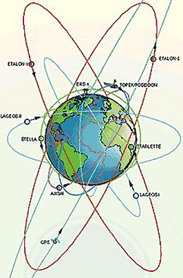
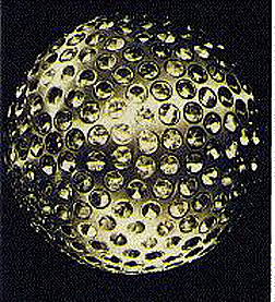
They have one thing in common: They all have corner-cube reflectors emplaced on their outer surface. These, and many other satellites, are used in a technology called Satellite Laser Ranging (SLR). This is the reverse of laser altimetry where the instrument transmitting the laser beam is on the satellite itself. Check this Website for a good review of the basic principles underlying SLR. In SLR, the laser generator is fixed at a ground station and its beam is directed into space to intercept and track the satellite equipped with silicon glass plates (usually two per port, mounted at right angles [corner-cube configuration] so as to accept a beam from any direction and return it) in an array termed retrograde reflectors. Here is Lageos (sometimes written as LAGEOS; it stands for Laser Geodynamics Satellite), one of the first satellites dedicated to geodesic measurements, orbited at 6000 km in 1976.
This schematic diagram synopsizes the mode of operation of a typical SLR system:

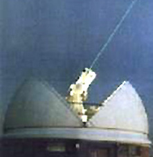
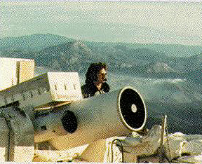
These are two of the now more than 46 active SLR stations in a global network:
The laser beam consists of coherent light generated at the site and sent out through a telescope as bursts of very short pulses. The beam seeks out an orbiting satellite and after finding it will continue to track the orbit for a time. A given pulse is returned to the SLR site in a very brief period of time; the time of start and the time of the same pulse’s return can be very precisely determined by a maser clock (interval differences in picoseconds [10:sup:-12 sec] can be separated). Since the speed of light is known very precisely, the distance between the SLR station and the satellite at the instant of intercept can be determined to an accuracy of less than a meter. Since separate ephemeris data can fix the position of the satellite quite accurately, the distance plus angle of beam projection allow the location of the station to be well set. (As an aside, the “trick” in the whole operation is to be able to “hit” the fast-moving satellite [whose size may be a meter or the mirror-bearing part of a larger satellite may be not much bigger], and then follow it; optical and radio [S-band; 10 cm wavelength] tracking or Doppler tracking allow the orbital path to be so exactly known that its position at any moment can predicted so closely that the chances of an intercept are quite good [and, typically, one in every 5 to 10 pulses will reach a mirror])
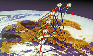
Commonly, a satellite is within the line of sight of several SLR stations. These may operate simultaneously such that they in effect “triangulate” on a satellite, a situation that greatly favors more accurate determinations of position, both of the satellite and the ground stations. Thus:
There are now a fair number of satellites fitted with retroreflectors suited to SLR tracking. Some of these have other prime purposes; a few are simply targets for geodetic studies. This next chart shows the past, presently functioning, and plannned satellites equipped with reflecting mirrors:
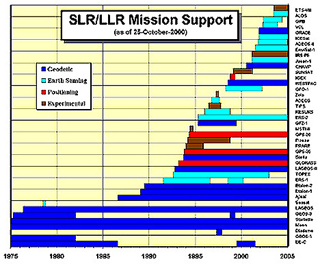
Because the lettering on the ordinate that identifies a satellite is hard to read, here is a partial listing of SLR-compatible satellites: ADEOS; ALOS; CHAMP; Envisat; ERS1 and 2; Etalon; Geos3; GLONASS; GPS35 and 36; Lageos1 and 2; Meteor3 and 6, Starlette; Stella. The designation LLR refers to Lunar Laser Ranging; three reflectors were left on the Moon’s surface by Apollo astronauts and two more were on Russian probes that successfully landed; their presence has allowed much improved determinations of the lunar orbit and distance variations. A list of satellites that participate in SLR measurements is found at this Goddard Website.
Notice that the listing includes two GPSs (Global Positioning Satellites). This is an entirely separate system for location of points on the Earth or in space (it is the basis of civilian commercial hand-held instruments that allow anyone to locate himself/herself on the ground [for instance, when hiking in the wilderness] or in a car or boat). The system in likewise invaluable as a surveying method and in conducting some of the studies mentioned in the next paragraph. More is said about GPS on page 11-6 or you can find a good review online at this University of Colorado summary site. The Russians operate a similar system called GLONASS.
The use of SLR has become sophisticated enough that its data are now collected and available through the International Laser Ranging Service. From these data are derived the International Terrestrial Reference Frame, a compilation of data on movements and relevant conditions of the land and ocean surfaces.
SLR has found many important applications, chief among which are: Polar motions and Earth rotations; gravitational variations of land surfaces; ocean surface configurations; ocean tides in basins; ice mass and volume; post-glacial rebound measurements; crustal deformation and tectonic plate motions.
This last category involves a major NASA, NOAA, U.S.Geological Survey program, joined by a group of international organizations that is commonly referred to as the Crustal Dynamics (now run out of Codes 920.2 and 926, NASA Goddard, check their Website); related information is found at the Geodynamics Branch site. The main objective is to measure both horizontal and vertical movements of the Earth’s tectonic plates and their influence on crustal deformation. These motions, particularly at plate boundaries, amount to a few millimeters to centimeters a year. By checking periodically every several years on the precise locations of geodetic control points, mainly at specific stations established as bench sites, the actual movements of these points translate into approximately the same displacements within the plates driven away from spreading ridges. Very precise measurement of these points as they shift over time has allowed reliable estimates of the movements (both direction and velocity) both within plates and at their edges. Different plates move at different rates and directions.
SLR has proved capable of high accuracy. But another method, Very Long Baseline Interferometry (VLBI), also is also able to pinpoint a station’s position and changes since its previous location(s). It relies on extremely accurate analysis of radio signals from distance sources that are received simultaneously at several radio telescope stations. Some of the basics of VLBI are covered at this Goddard site. The Canadians have prepared another good review site covering Principles of Radio Interferometry; a clear overview of some general principles of interferometry is found at this Canadian site.
Some of the main ideas behind radio interferometry are summarized here. Look first at this diagram:

The radio wave source is usually some radio galaxy or a quasar sending strong radio signals. These, of course, travel at light speed. Two or more widely separated (very long baseline; resolution increases with length or separation) radio telescope receivers each record the signal. Each is also tied to a very accurate (hydrogen maser) clock which synchronizes the timing. Data reduction includes removing atmospheric effects and then checking time differentials for a given signal which result because one station is further away from the distant signal source than the other. The wave forms of the signals thus do not coincide precisely, i.e., they show partial to complete constructive or destructive interference (in optical interferometry, these slight differences in phase would appear as light fringes). Using a computer-based correlator, signal analysis by cross-correlation is conducted, as displayed in this diagram:
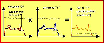
The result is a new data set from which the positions of reference points can be calculated and compared. Presently, about 40 receiver sites, mostly in North America and Europe, are participating in this effort.
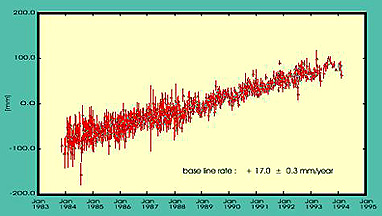
The most accurate data on displacement rates comes from averaging years of measurements. For instance, this plot covers 10 years of continuing data for the increasing separation between a European and a North American station. While there is scatter (uncertainty) for each measurement, the straight line fit (17 mm/yr) is credible.
Two maps indicate the emerging patterns of relative plate motion for those plates with enough site points to indicate both magnitude and direction of movement. The first is more general:
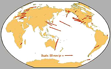
The plate containing the European “continent” is moving northeast, as the African plate pushes against it. The Pacific plate’s direction is to the northwest. Two contrasting movement patterns occur in the North American plate; most is being driven west from the Mid-Atlantic Ridge but a small segment in western California southward is moving north-northeast where complex interactions with the eastern Pacific plate cause sliding along a series of transverse faults (e.g., San Andreas). This next diagram offers more details and shows the fastest movements now occur in California and in southeast Australia.
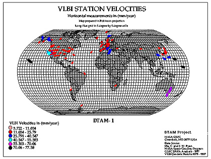
This is more evident in the following map on which velocity vectors are plotted relative to the plates involved:

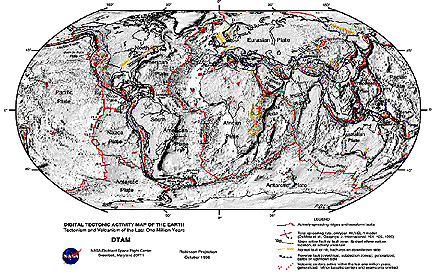
One of the by-products from NASA Goddard’s Geodynamic Branch work on crustal deformation is the splendid plate tectonics map made by Dr. Paul D. Lowman, Jr. (author of Section 12 of this Tutorial). It now shows plate locations, plate velocities, and volcanic activity for the last one million years. We show this important map below but because at this smaller size it is unreadable we offer the option of looking at a large, more readable version by clicking here (to return to this page, hit your Back button).
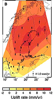
Crustal movements of another kind have now been further detailed using positional information obtained from ranging to the Global Positioning System array of satellites. Parts of the Earth’s crust were depressed (pushed downwards) from the weight of several kilometers thickness of ice at various times during the Pleistocene Ice Ages. As the more rigid upper crust bends down, the more plastic lower crust/upper mantle is driven sidewards to make room. When the ice sheets melt, there is a slow, generally steady upwards rebound that is now being measured by GPS and other satellites. A group of scientists at the University of Toronto and other institutions have recently reported on results obtained for the Fennoscandinavian crust. The illustration on the left shows measured vertical rebound; that on the right indicates that these workers also detected some horizontal movement outward from a depression center.

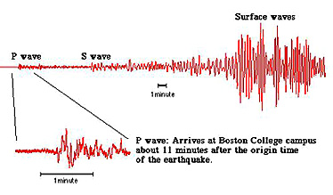
The third major subdivision of applied geophysics, Seismology, obviously does not benefit directly from space observations. Seismometers must of necessity be on the surface, preferably mounted on bedrock, to pick up the various kinds of seismic disturbances, especially from earthquakes. The seismic waves are oscillations of several types - P or primary waves (push-pull [compressional], analogous to acoustic wave motion), S or secondary waves (sinusoidal, also called shear waves), and others, such as surface Love and Rayleigh waves. Each wave type travels from its source to a seismic monitoring station at some velocity, dependent on its depth and the seismic properties of materials along its particular path to the station. The oscillations at the station are recorded as “wiggles” or tracings on a seismogram. Here is a seismogram recorded at the Weston Station of Boston College for a recent earthquake in Turkey. The seismic waves traveled first through the crust under Turkey, then the Upper Mantle, and finally through the crust of the North American Plate under Boston.
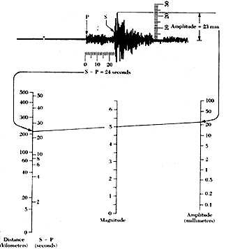
Much can be learned from a seismogram: the distance to the earthquakes epicenter (point at the surface about its zone of origin); depth to the origin; magnitude or intensity (and kinetic energy released); duration; direction of movement; and often the type of fault along which the earthquake movement results in strain release. Each station has developed nomographs that can be used to solve for some of these parameters. Examine this one:
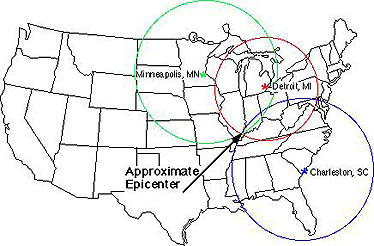
The distance to the epicenter can be in any direction (360°) from the station. But when distance information from three stations is used to draw a circle from each with the radius taken as its distance to the epicenter, there will emerge a narrow zone of intersection that defines the epicenter common to the three; thus:
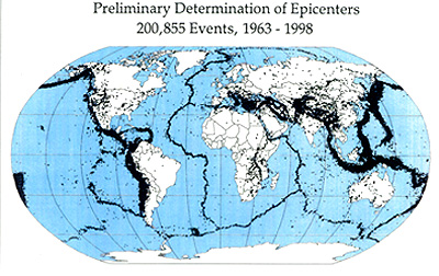
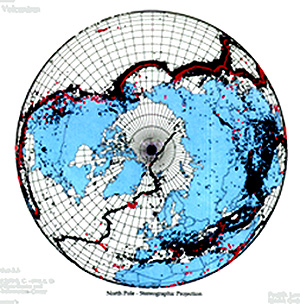
Over many decades of record keeping, thousands of epicenters have been plotted over the entire world. Here is a map produced by Paul Lowman and colleagues showing these epicenters; note that the vast majority concentrate near plate subduction zones (where one plate dives under another at a convergent boundary) or at spreading ridges.
Seen from the viewpoint of looking down at the northern hemisphere (North Pole at center), and with zones of active volcanism in red and continents in blue, the pattern again reveals that most earthquakes and volcanic eruptions occur at plate boundaries.
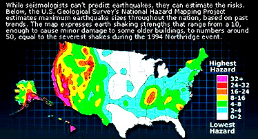
Such plots help to define zones or regions of higher earthquake activity. This distribution plus information about the nature and extent of damage allows estimates of seismic risk or likelihood of degree of destruction within some time span. This risk map has appeared in the newspaper USA Today shortly after an earthquake in Seattle, Washington in late February of 2001.
As said above, satellites cannot directly record earthquake (seismic) events. However, some seismometers are located in isolated places where direct telephone lines do not reach. Transmitters at the field station can telemeter data to satellites overhead that then relay the recorded seismic signals to receiving stations. Magnetic or gravity measuring satellites do reveal much about the Earth’s interior which is of use in interpreting internal conditions related to plate motions that are factored in models used to analyze earthquake mechanisms.
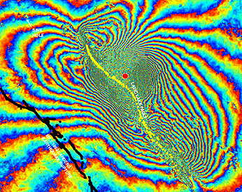
There is one other use of satellites that bears on earthquake effects. This employs radar interferometry to examine displacements of the surface (SLR and altimeter profiling also can contribute to determining changes in surface position and elevations brought on by an earthquake). Color fringes produced from interferometric data indicate the distribution of changes in the surface (data from a pre-earthquake passage of the satellite are used to work out the differences in position).
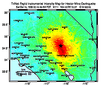
An excellent case study which used this technology is the 7.1 magnitude Hector Mine earthquake of October 16, 1999 40 km northwest of Barstow, California (edge of Mojave Desert). This map shows the intensity distribution (relates to how people perceived the quake) around the epicenter.
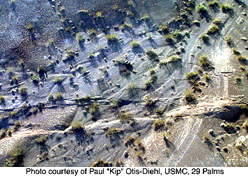
This quake occurred in what is known as the Mojave shear fault zone. Lateral displacement along this predominantly strike-slip fault ranged from 3.8 to 4.7 meters (almost 15 ft). Surface rupture extending for 41 km can be seen in this aerial photo taken near the mine; the offset road (right) reveals this displacement.
Here is an interferogram (displayed by color fringes) showing displacement strain along surface around the Lavic Lake fault which triggered the Hector Mine earthquake, as determined from analysis of SAR data from the ERS-1 satellite:
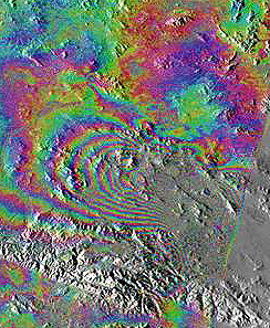
A similar plot, superimposed on an image background, shows vertical displacement after an earthquake near Landers, California in the Mojave Desert. This occurred in 1992 within the same shear zone as the Hector Mine earthquake.
In these three pages, we have only “scratched” the surface (no pun intended) on how space technology contributes to the geophysical characterization of the Earth and its environs. Much more can be garnered from surfing the Net. NASA’s Goddard Space Flight Center has an index and links to many sites that tell the story of how various geophysical methods are revealing much that is new, or continually monitoring on-going studies, about nearly all aspects of geophysics.
This subsection on geophysics as a component of remote sensing in its broadest meaning is, from what you have seen, a worthy diversion from the main theme. We move on to that theme - the more customary types of remote sensing - in the rest of this Introduction and the Sections that follow, first by investigating the role of the photon and its place in determining the characteristics of the electromagnetic spectrum.