Other Remote Sensing Systems - Radar and Thermal Systems
Contents
Radar (an active microwave system) has been flown on both military and civilian spacecraft because of its ability (for certain wavelengths) to penetrate clouds. Seasat, the SIR series, and Radarsat are among the instruments used so far. Thermal remote sensing, operating primarily in the 8-14 µm but also in the 3-5 µm wavelength region of the spectrum produces diagnostic data that can aid in identifying materials by their thermal properties. Some meteorological satellites have thermal sensors, as does the Landsat TM. A multispectral thermal scanner, TIMS, is described.
Other Remote Sensing Systems - Radar and Thermal Systems
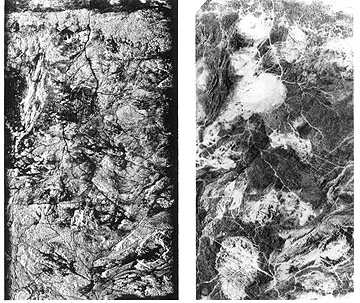
Another class of satellite remote sensors now in space are radar systems (these are treated in detail in Section 8). Radar commonly provides a very different view of the same landscape compared with a visible image. This is obvious in this pair showing an ancient terrain in Egypt with fractures in a crystalline terrain evident in the left image (SIR-A radar) and plutons in the same scene in the Landsat image on the right.
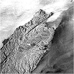
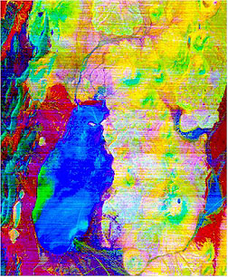
The first civilian radar system to operate from space was mounted in a Space Shuttle. Seasat was an experimental L-Band radar whose primary mission was to measure ocean surfaces. However, it produce very informative images of the land surface, including this scene that includes Death Valley, one of the prime test sites for determining the capabilities of various sensors.
|Seasat radar image of Death Valley, California and surrounding mountains. |
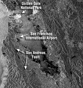
` <>`__I-26: Look at the above two radar images, especially the one showing San Francisco. State two characteristics of the radar images that seem to differ from those of Landsat. **ANSWER**
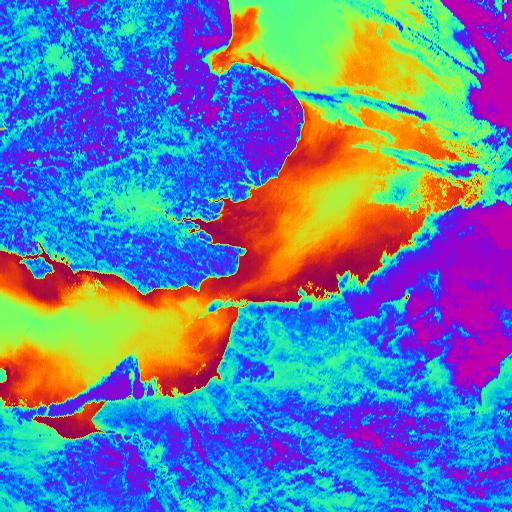
The ERS satellites had other sensors, as was indicated in the Overview. One in wide use is ATSR (Along Track Scanning Radiometer). Here is an image of the English Channel made by that instrument:
NASA, through its Jet Propulsion Laboratory (JPL) in Pasadena, California, has flown three radar missions on the Space Shuttle. The SIR (Shuttle Imaging Radar) series has used different wavebands and look conditions, with many excellent images over much of the globe having been acquired. Appearing below is a SIR-C image obtained on October 3, 1994 during a flight of the Space Shuttle. This is a false color composite made by assigning the L-Band HV, L-Band HH, and C-Band images to red, green, and blue respectively (see page 8-7). The area shown is that part of Israel containing disputed West Bank territory that includes Jerusalem (yellowish patterns on left) and the top of the Dead Sea.

Remote sensors that cover two thermal intervals - the 3-5 µm and 8-14 µm broad bands (corresponding to two atmospheric windows) allowing sensing of thermal emissions from the land, water, ice and the atmosphere - have been flown on airplanes for several decades. Many of the meteorological satellites (see next page) include at least one thermal channel. A thermal band is included on the Landsat Thematic Mapper.
The principles behind thermal remote sensing are treated in some detail in Section 9. For now, let us look at two representative samples of the types of thermal images that indicate the kinds of information resulting from operation of thermal sensors on moving platforms above the Earth’s surface.
This next image was made from a satellite dedicated to sensing one thermal property - thermal inertia (defined on page 9-3). The Heat Capacity Mapping Mission (HCMM) was launched in 1978 and is described on page 9-8. This image covers about 700 km (435 miles) on a side and was taken at night (daytime thermal images were also generated) on July 16, 1978 over southern Europe using a sensor that integrates thermal emissions within the wavelengths from 10.5 to 12.5 µm. The darker area in the upper left portrays lowlands in eastern France and southwestern Germany. The Alps form a broad arc crossing the image. The blackish pattern within the Alps corresponds to the cold higher elevations (with some snow). The lighter-toned land below the Alps is the Piedmont and western plains of Italy’s Po Valley. The light tones near the image bottom are the waters of the Mediterranean Sea, which at night are warmer (heat sink) than most land surfaces.

Thermal data, especially from the 8-14 µm region become more valuable in singling out (classifying) different materials when this spectral interval is subdivided into bands, giving multispectral capability. NASA’s JPL has developed an airborne multiband instrument called TIMS (Thermal IR Multispectral Scanner) that is a prototype for a system eventually to be placed in space. The images it produces are notably striking in their color richness, as evident in this scene that includes a desert landscape around Lunar Lake in eastern California.
The image pair below covers a part of the White Tank Mountains of Arizona. The left image is made from 3 TIMS bands; the right is a false color composite formed from visible band data on another multispectral scanner onboard the aircraft that gathered TIMS emitted radiation.
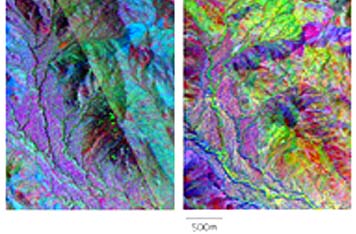
While these color patterns make some sense when interpreted through geologic maps, aerial photos, field visits (ground truth), etc., it is hard to envision what they mean just from this image pair. Perhaps a better insight and context will result from the view below, which is an oblique or perspective “photo” showing the full extent of the White Tank Mountains (a fault block range) and surrounding desert and agricultural farms, about 40 km (25 miles) west of Phoenix. But, this is really a “trick picture”, in that it is made from Landsat TM bands (1,2,3) that have been registered to Digital Elevation Model (DEM) data (see page 11-5) that contain heights above sea level, from which a 3-dimensional representation is constructed. Other such examples will appear in several Sections of this Tutorial.
