TIROS and Nimbus
Contents
The historical background leading up to the launching of fleets of meteorological satellites is briefly touched upon. The first U.S. group, the TIROS series, is described. Greater discussion of the Nimbus program, including a table listing the various instruments used in the series still flying, expounds upon its accomplishments. Instruments singled out for illustrative examples are: HRIR; IDCS; SCMR; ESMR; SMMR; TOMS; and SBUV; other sensors are mentioned. NOAA satellites are mentioned here if they supported any of these sensors.
The United States metsat program traces its formal inception to the launch of Vanguard 2 in February of 1959, just 12 months after our first ever successful satellite, Explorer 1. The spacecraft failed because of a wobbly attitude. An improper orbit on the next attempt, with Explorer 6, led to a few low resolution pictures of Earth. NASA achieved success with Explorer 7, orbited on October 13, 1959, which carried a radiometer designed by Verner Suomi, America’s pioneer in satellite meteorology, and his colleagues. Using black and white hemispheres on the sensor to calibrate, this instrument measured solar and terrestrial radiative energy (determining reflective and absorbed components) to estimate radiation balance.
TIROS and Nimbus
The first experimental meteorology series began with TIROS-1, launched on April 1, 1960. TIROS stands for Television and Infrared Observational Satellite. The main instrument was a vidicon, which is a modified television camera that scanned through 500 lines, each containing 500 pixels. Although desinged to function primarily to learn what that kind of satellite can contribute to meteorology, TIROS (and Nimbus) both provided useful insights as well into land observations for earth resources applications.
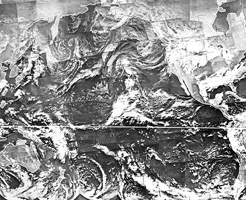
We show here one of the nearly 23,000 images returned from TIROS-1:

` <>`__14-8: Why is there a blocky disjointedness associated with this image?` <Sect14_answers.html#14-8>`__**ANSWER**

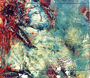
Nimbus-1, launched on August 28, 1964, was the first that were put in a sun-synchronous orbit (now the norm). It used a three-axis stabilization technique (based on flywheels) that kept it pointed constantly at Earth. It carried several instruments including the Advanced Vidicon Camera System (AVCS, an APT) and the High Resolution Infrared Radiometer (HRIR), which operated in the 3.6-4.2 µm interval. An example of a Nimbus 1 HRIR image, taken at night over western Europe, appears next, on the top (note the distortion that enlarges Germany and Sweden relative to southern countries-the Italians may be aggrieved by the shrinking of their “boot”!). On the bottom is a visible Image Dissector Camera System (IDCS) image of the southeast U.S., as seen by Nimbus 3:

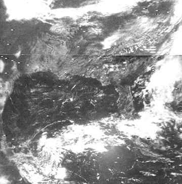
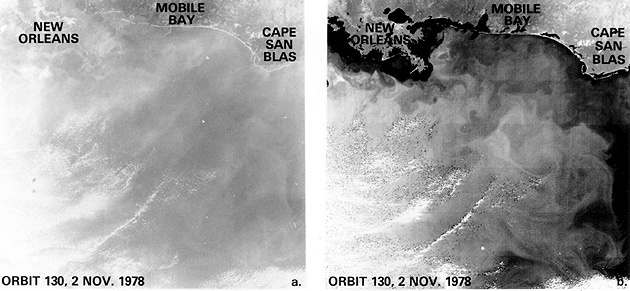
` <>`__14-9: The thermal image shows extended groups of swirly white patterns. Are these clouds or thermal patterns in the Gulf of Mexico seawater? Cite a logical clue to your conclusion. **ANSWER**
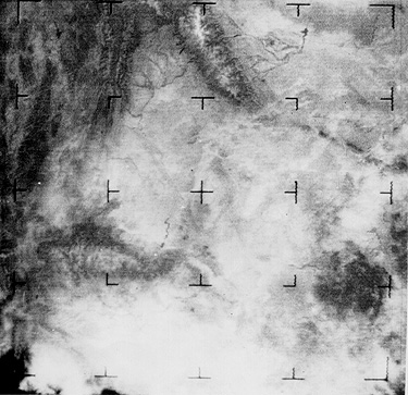
The basins generally are highly reflective, and the mountains tend to stand apart because of dark tones associated with evergreen vegetation. Compare this image with the Landsat 1 MSS mosaic of the entire State of Wyoming that was made for me (NMS) as part of my Wyoming project as a Co-Investigator with the Geology Department at the University of Wyoming:
` <http://wtlab.iis.u-tokyo.ac.jp/wataru/lecture/rst/Sect2/nicktutor_2-8.html>`__.
14-10: This Nimbus image was the first remote sensing product ever worked on by the writer (NMS) when I transferred in 1970 from the planetary to the remote sensing programs at NASA Goddard Space Flight Center. Then, I took the Landsat mosaic into the field a few months after that satellite sent its first pictures in July of 1972. Just for fun, why don’t you fit the Nimbus image into the Landsat mosaic - and check the answer. **ANSWER**
Nimbus 3 (April 14, 1969) also was the first to use atmospheric sounders extensively, with its Infrared Interferometer Spectrometer (IRIS ), operating between 6 µm and 25 µm and Satellite Infrared Spectrometer (SIRS ), sensing in the 15 µm region. Nimbus 4 (April 8, 1970) carried the Backscatter Ultraviolet (BUV ) radiometer, becoming the first metsat to measure atmospheric ozone.
Two instruments on Nimbus 5 (December 11, 1972) are of special significance. The Surface Composition Mapping Radiometer (SCMR) uses two thermal bands, 8.4-9.5 µm and 10.2-11.4 µm, to produce color-coded temperature maps, such as this image of Florida and Cuba and surrounding waters, made from the 8.8 µm channel:
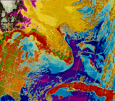
Ratios of radiant temperatures measured by the two bands provide a qualitative estimate of SiO2 content of rocks and soils. This process uses the concept of “restrahlen”, a German term that refers to decreased emissivity because of resonance vibrations associated with silicon-oxygen bonds in silica tetrahedra. As the silica content increases, the emissivity decreases more and also shifts as wavelengths become longer.
` <>`__14-11: How might this silica shift be used practically? **ANSWER**
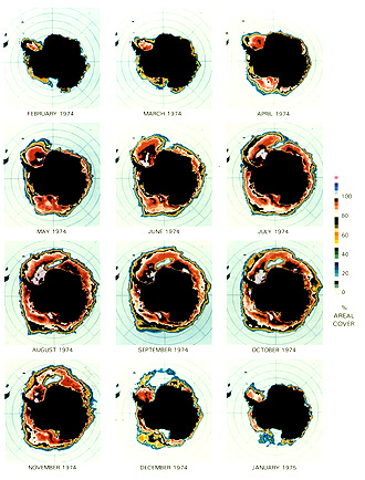
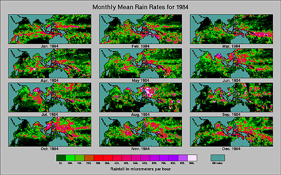
The Electronically Scanning Microwave Radiometer (ESMR ) on Nimbus-5 operated at a 19.35 GHz frequency (1.55 cm wavelength) to sense brightness temperatures of the surface and atmosphere. This instrument was capable of sensing surface ice temperatures, especially in the polar regions, as shown in this time series of maps that plot the percentage of ice cover around Antarctica on a monthly basis in 1974. The ESMR was also the first to use microwave absorption to estimate precipitation (rain rates) by quantifying increases in optical depth, which correlate to higher brightness temperatures. The ESMR on Nimbus 6 (June 12, 1975) was set at 37 GHz (0.81 cm).
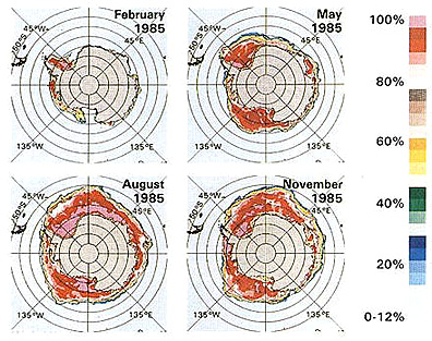
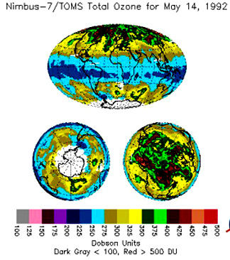
(Note: A Dobson unit is the response at 4 wavelengths by a Dobson spectrometer from which the total ozone from ground to the outer atmosphere can be measured and then recalculated as a compressed column of ozone equivalent to a 0.01 mm thick, measured over a fixed area centered on Labrador in eastern Canada and adjusted to a STP of 1 atmosphere and O° C.)
In the above maps, the ozone content is higher in high latitudes in springtime. The lower values closer to the equator are of concern because high ozone content affords greater protection from harmful UV radiation.
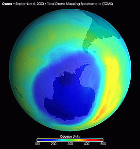
The South Polar ozone hole has grown wider since 1992. Here is a TOMS image of much of the southern hemsphere, centered on Antarctica, which in September, 2000 disclosed the largest expanse of high ozone levels yet recorded; the hole since has shrunk a bit.
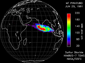
We can also use the TOMS to monitor SO2 in the atmosphere. After some major volcanic eruptions, it tracked extensive clouds of SO2-enriched ash and gases injected into the upper atmosphere daily across much of the world, until they dissipated below detection levels. Here is the status on June 20, 1991 of the cloud produced by the Mt. Pinatubo eruption in the Philippines.
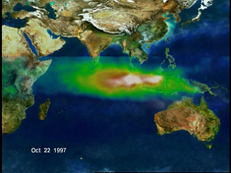
TOMS has proved very useful in monitoring other kinds of atmospheric disturbances such as massive smog buildups that persist over time. Forest fires in Indonesia and elsewhere from September through November of 1999 led to a huge elongate trail of gases that were carried by winds westward to Africa. This TOMS image should the smog and associated clouds near its maximum extent:/p>
The first Solar Backscatter UltraViolet (SBUV) sensor was on Nimbus 7 (also SBUV/2 on NOAA-9, -11, and -14), sharing some of the components of the TOMS. The SBUV had 12 channels in the UV region providing coverage between 160 and 400 nm. Shown below is a SBUV/2 map of ozone distribution (in Dobson Units) for the South Polar (Austral) Spring. Then, beneath that are graphical data sets for areas of coverage in that region for the months of September through December of the years 2000 and 1999, and three curves summarizing grouped data for 1990-99:
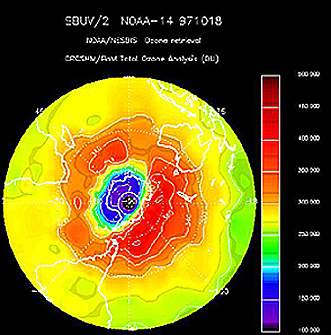
|Areal extent of the austral ozone hole for the months and years indicated; SBUV data. |
Both the TIROS and Nimbus programs were initiated by NASA. Later ones in the two series included NOAA as a major participant and eventual operator.
Primary Author: Nicholas M. Short, Sr. email: nmshort@nationi.net