CZCS and SeaWiFS
Contents
The oceans teem with life but of course fish and even whales are not resolvable by the usual satellite sensors. But sealife has to eat and at the base of their foodchain is microscopic plant and animal life known as plankton. Algae, in particular, are fundamental food (even for whales). Being marine plants, they experience the same responses to light owing to chlorophyll content (absorbing in the blue and red). Satellites can determine plankton content by analyzing the color variations (mainly in the visible) of seawater inasmuch as much of the color changes correspond to presence of life. Two satellites, the Coastal Zone Color Scanner (CZCS) on Nimbus 7 and SeaWiFS provide valuable data on ocean color. This translates into practical information for the fisheries industry. Satellite sensors also are very effective in scoping the patterns of sediment distribution, using mainly the Vis-NIR bands.
CZCS and SeaWiFS
The world’s oceans (and its freshwater bodies, as well) teem with life. Central to the marine foodchain is phytoplankton - microscopic plants that photosynthesize chemicals in sea water. This process depends on the plankton content of chlorophyll a, a pigment that strongly absorbs red and blue light. As plankton concentrations increase, there is a corresponding rise in spectral radiances, peaking in the green. Upwelling masses of water (usually associated with thermal convection) containing phytoplankton take on green hues in contrast to the deep blues of ocean water with few nutrients.
The Coastal Zone Color Scanner (CZCS) is a sensor specifically developed to study ocean color properties. It launched in October 1978, as part of Nimbus-7’s instrument complement and continued to operate until late 1986. It sensed colors in the visible region in four bands, each 0.02 µm in bandwidth, centered at 0.44 (1), 0.52 (2), 0.57 (3), and 0.67 (4) µm. A fifth band between 0.7 and 0.8 µm monitored surface vegetation and band six, at 10.5-12.5 µm sensed sea surface temperatures. In monitoring ocean color, band 1 (blue) measured chlorophyll absorption; band 2 (green), tracked chlorophyll concentration; band 3 (yellow), was sensitive to yellow pigments (“gelbstoff”); and band 4 (red), reacted to aerosol absorption. With data from those bands, we calculate the chlorophyll variation, which correlates closely with relative abundance of marine phytoplankton, as the ratio of band 1 to band 2 (for phytoplankton concentrations less than 1.5 mg/m3) and band 2 to band 3 (>1.5 mg/m3)
A good users guids for how to use CZCS and similar data sets is found in this CZCS Starter Kit.
The next pair of images are CZCS color composites: the left one emphasizes chlorophyll-enrichment (in reds) in the Georges Bank off the New England coast (BGR = bands 3,2,1) whereas the right one simulates natural ocean color (BGR = bands 1,2,3)
|Left:CZCS color composite showing the distribution of strong chlorophyll (mainly plant life) off the Georges Bank of New England and Nova Scotia; June 6, 1979; Right: Same scene now rendered in natural color. |
<originals/Fig14_82.jpg>`__

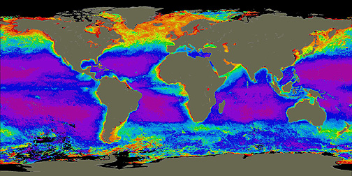
` <>`__14-33: These chlorophyll distribution maps show concentration gradients that seem to run counter to logic (or intuition), in that the lowest amounts of chlorophyll (hence plankton) are in the equatorial and subtropical zones. Those zones, being warmer, should support greater quantities of plant life (as do the tropics on land). What gives here? **ANSWER**
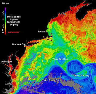
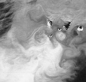
In the color coding, blues correspond to the lowest levels of phytoplankton and reds to the highest. Thermal data as such are not directly contributing to the color composite of this image but notations about warm and cool areas in the water result from thermal data from another satellite. Note the eddies or rings. Phytoplankton tends to concentrate along the edges of warm core rings (which rotate clockwise) but concentrate centrally in cold core rings (counterclockwise motion). The motions in these rings are analogous to circulation around atmospheric high- and low-pressure systems. Warm core rings can extend over several hundred kilometers, as seen in this HCMM, Night-IR, thermal image (left or top), which shows such “gyres” in varying stages of development and coherence in Atlantic waters near the Canary Islands off the African coast. Cold core rings are usually less well shaped but are probably displayed in this June 19, 1976, Landsat-1 band 4 (green) image (right or bottom) of waters off the southwest coast of Iceland; concentrations of phytoplankton are associated in part with the lighter tones that may also be tied into sediment “murkiness”.
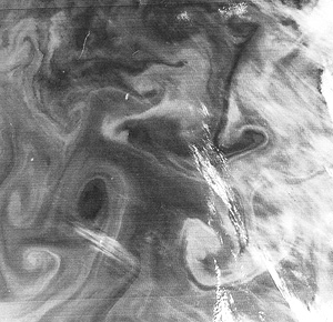
` <>`__14-34: Which way do the eddies seem to be rotating in the above two images? **ANSWER**
These observations types - ocean color and thermal patterns - aid in locating conditions where large schools of fish are likely to live, so commercial and sport fishermen actively apply them to locate the best current fisheries.
The follow-on to the CZCS is NASA Goddard’s SeaWiFS (Sea-viewing Wide Field-of-View Sensor), launched successfully on August 1, 1997. It is the prime sensor on a commercial satellite, Orbview-2 (originally named SeaStar) operated by the Orbital Imaging (OrbImage) Corporation. Once again, the sensor system monitors ocean color variations, especially those caused by concentrations of plankton and other sealife that strongly moderates chlorophyll response, detectable spectrally. Thus, the prime objectives are: 1) to quantify ocean plankton production; 2) to determine observable couplings of physical/biological processes; and 3) to characterize estuarine and coastal ecosystems. We show the prime sensor here:
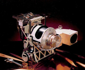
The SeaWiFS sensor consists of eight channels at: 412, 443, 490, 510, 555, 670, 765, and 865 nm (nanometers: 1µm = 1,000 nm), each with bandwidths of 20 or 40 nm. The instrument can swing ±58° off nadir. From an orbital altitude of 705 km (438 mi), spatial resolution in the Local Area Coverage (LAC) mode is about 1.1 km (0.68 mi) (the optimal resolution is 0.6 km at nadir), and in the Global Area Coverage (GAC) mode, it is 4 km (2.5 mi). Swath widths are: LAC = 2,801 km, and GAC = 1,502 km. Further information about this instrument (plus additional images) is available online at: SeaWiFS.
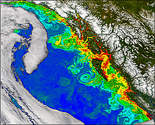
Like CZCS, SeaWiFS produces regional scale images in which eddies and circulation patterns are evident. In this view of the western North American continent, marine eddies have formed off the British Columbia coast around Queen Charlotte; to the west is still another eddy-like pattern made by clouds.
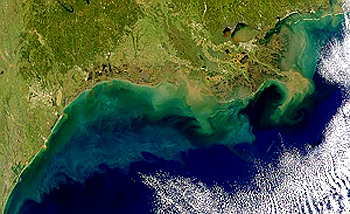
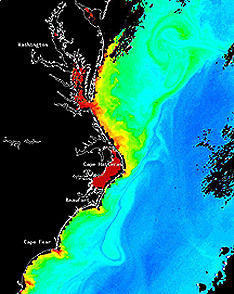
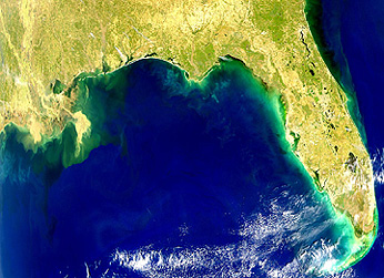
One job that SeaWiFS does well is to monitor sedimentation patterns. Below is an image of the western Gulf of Mexico, showing sedimentation either in browwn or in green (much lower concentrations of sediments, but enough to modify water color to lighter tones). (Tie this image with that four illustrations down.)


Chlorophyll response is also strong in floating algae. The Red Tide is a much dreaded form of algae that secrets and expels a poison that can be fatal to fish and shellfish such as oysters. This SeaWiFS image of the northeastern Gulf of Mexico shows (in light blue-green) a nearshore concentration of this algal bloom on March 1, 1999:
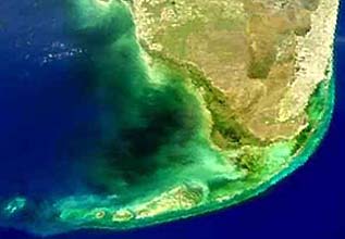
In Winter of 2002, another algal bloom of a different nature affected the eastern Gulf of Mexico north of the Florida Keys. The seawater became black for a while, then reverted to a brownish-green. The bloom extended over a larger area than customary. From a boat, the water indeed appeared black. Fish within the bloom were not killed but nevertheless left the area until the algae died off. Here is a SeaWifS image of the bloom at its height:
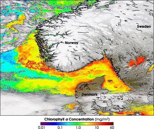
SeaWiFs has produced a striking image that shows algal blooms from plankton, in amounts related to chlorphyll count, in the Baltic Sea and Atlantic Ocean off Norway and adjacent countries:
Plankton concentration (as revealed by its chlorophyll signature) is very sensitive to water temperatures. Thus, significant temperature changes in tropical waters associated with the El Niño event during the late 1990s can the controlling factor in plankton distribution, as indicated by these two SeaWIFS images in May of 1998, in which plankton appear in profusion (expanded right inset) as temperatures drop in the area it represents:
temperature variations, as determined by SeaWIFS.|
` <>`__14-35: Imagine you are a commercial fisherman. How would you use satellite imagery to find the best fishing grounds? **ANSWER**
We can also use the sensor data from SeaWiFS to map land surfaces on a local to global scale. We showed a global, true-color map of Earth near the end of the Introduction Section. This next SeaWIFS image depicts still another use for the meteorological/oceanographic class of satellites by monitoring a dust storm coming off the northwest Sahara desert of Africa as it blows out to sea:

ADEOS, that ill-fated but most promising multisensor satellite, had two instruments that could perform ocean color and phytoplankton assessments. First below is a January 1997 global image made by the OCTS (Ocean Color and Temperature Scanner) and beneath it is a April 1997 view of the Mediterranean made by POLDER.

As has been seen in several images elsewhere in the Tutorial, sensors operating mainly in the 0.4 to 0.7 µm spectral interval are capable of monitoring the distribution of sediments (current-driven) in circulation or even in standing water. The density of sediment in the waters very near the surface can be quantitatively assessed. In practice, on-site measurements can provide calibration points to determine densities. Here is an example of the determination of variations in sediment density in the San Francisco Bay and off the coast of the Peninsula there, as measured by Terra’s ASTER (see also page 16-10 for complementary images).
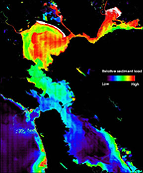
The higher densities in the northern S.F. Bay and adjacent San Pablo Bay are due to sediment being carried into these waters from the Sacramento River.