Some Basic Image Processing Procedures
At this point we turn to a more intense examination of computer-based procedures for working with the digital data acquired by remote sensors. The three general types of image processing are introduced. The programs that convert the raw DN values from individual bands into photographs or computer displays often yield visually poor products, especially if there is a narrow range of DN�s and/or an even narrower range dominates as a single histogram peak. This is improved, often greatly, by applying standard or specialized processing procedures. On this page, the first step in optimizing the data, especially for pictorial purposes, in called Preprocessing.
Some Basic Image Processing Procedures
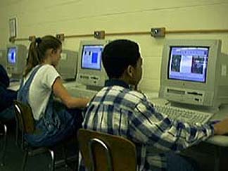
The roots of remote sensing reach back into ground and aerial photography. But modern remote sensing really took off as two major technologies evolved more or less simultaneously: 1) the development of sophisticated electro-optical sensors (see page I-5a) that operate from air and space platforms and 2) the digitizing of data that were then in the right formats for processing and analysis by versatile computer-based programs. Today, analysts of remote sensing data spend much of their time at computer stations, as shown below, but nevertheless still also use actual imagery (in photo form) that has been computer-processed.
Now that you have seen the individual Landsat Thematic Mapper (TM) bands and color composites that have introduced you to our study image, we are ready to investigate the power of computer-based processing procedures in highlighting and extracting information about scene content, that is, the recognition, appearance, and identification of materials, objects, features, and classes (these general terms all refer to the specific spatial and spectral entities in a scene). A very helpful summary of the main ideas involved in digital image processing is provided in Volume 3 in the Remote Sensing Core Curriculum first cited in the Overview of this Tutorial. Jan Husdal has produced a good Internet site worth visiting for more on image processing (but it may “stick” on screen after you try to leave via the “Back” button). Another useful overview tutorial has been put on line by the Chesapeake Bay Institute at Towson University in Maryland. Chapter 7 on Image Processing, from Floyd Sabins, Jr.’s excellent text on remote sensing, has been reproduced online at this site. There is also some helpful supplementary ideas on basic processing in the first five pages of Appendix B of this Tutorial.
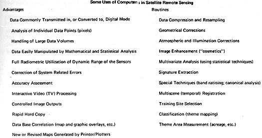
The advantages of computer processing and the common routines or methods are summarized in this Table:
Processing procedures fall into three broad categories: Image Restoration (Preprocessing); Image Enhancement; and Classification and Information Extraction. The first of these is considered on this page. We will discuss on the next two pages contrast stretching, densing slicing, and spatial filtering; producing stereo pairs, perspective views, and mosaics are considered in other Sections of the Tutorial. Under Information Extraction, ratioing and principal components analysis have elements of Enhancement but lead to images that can be interpreted directly for recognition and identification of classes and features. Also included in the third category but treated outside this Section is Change Detection. Pattern recognition is often associated with this category.
A word about a parameter we have mentioned before (e.g, first on page I-5a and at the beginning of this Section), namely the meaning of the term Digital Number or DN. We have said that the radiances, such as reflectances and emittances, which vary through a continuous range of values are digitized onboard the spacecraft after initially being measured by the sensor(s) in use. Ground instrument data can also be digitized at the time of collection. Or, imagery obtained by conventional photography is capable of digitization. A DN is simply one of a set of numbers based on powers of 2, such as 26 or 64. The range of radiances, which instrument-wise, can be, for example, recorded as varying voltages if the sensor signal is one which is, say, the conversion of photons counted at a specific wavelength or wavelength intervals. The lower and upper limits of the sensor’s response capability form the end members of the DN range selected. The voltages are divided into equal whole number units based on the digitizing range selected. Thus, a Landsat TM band can have its voltage values - the maximum and minimum that can be measured - subdivided into 28 or 256 equal units. These are arbitrarily set at 0 for the lowest value, so the range is then 0 to 255.
Preprocessing
Preprocessing is an important and diverse set of image preparation programs that act to offset problems with the band data and recalculate DN values that minimize these problems. Among the programs that optimize these values are atmospheric correction (affecting the DNs of surface materials because of radiance from the atmosphere itself, involving attenuation and scattering); sun illumination geometry; surface-induced geometric distortions; spacecraft velocity and attitude variations (roll, pitch, and yaw); effects of Earth rotation, elevation, curvature (including skew effects), abnormalities of instrument performance (irregularities of detector response and scan mode such as variations in mirror oscillations); loss of specific scan lines (requires destriping), and others. Once performed on the raw data, these adjustments require appropriate radiometric and geometric corrections.
Resampling is one approach commonly used to produce better estimates of the DN values for individual pixels. After the various geometric corrections and translations have been applied, the net effect is that the resulting redistribution of pixels involves their spatial displacements to new, more accurate relative positions. However, the radiometric values of the displaced pixels no longer represent the real world values that would be obtained if this new pixel array could be resensed by the scanner (this situation is alleviated somewhat if the sensor is a Charge-Coupled Device [CCD]; see Section 3). The particular mixture of surface objects or materials in the original pixel has changed somewhat (depending on pixel size, number of classes and their proportions falling within the pixel, extent of continuation of these features in neighboring pixels [a pond may fall within one or just a few pixels; a forest can spread over many contiguous pixels]). In simple words, the corrections have led to a pixel that at the time of sampling covered ground A being shifted to a position that have A values but should if properly located represent ground B.
An estimate of the new brightness value (as a DN) that is closer to the B condition is made by some mathematical resampling technique. Three sampling algorithms are commonly used:

In the Nearest Neighbor technique, the transformed pixel takes the value of the closest pixel in the pre-shifted array. In the Bilear Interpolation approach, the average of the DNs for the 4 pixels surrounding the transformed output pixel is used. The Cubic Convolution technique averages the 16 closest input pixels; this usually leads to the sharpest image.
Because preprocessing is an expansive topic that requires development of a broad background, we will omit further discussion here. Instead, we refer you to any of the textbooks listed in the Overview and in Appendix B that treat this subject in more detail.