Supervised Classification
Contents
The principles behind Supervised Classification are considered in more detail. The fact that the pixel DNs for a specified number of bands are selected from areas in the scene that are a priori of known identity, i.e., can be named as classes of real features, materials, etc. allows establishment of training sites that become the basis of setting up the statistical parameters used to classify pixels outside these sites. The process by which training sites were selected for the Morro Bay scene, together with a plot of spectral signatures and a table of statistical means and site sample sizes illustrate the preparatory phase involved in this mode of classification.
Supervised Classification
Supervised classification is much more accurate for mapping classes, but depends heavily on the cognition and skills of the image specialist. The strategy is simple: the specialist must recognize conventional classes (real and familiar) or meaningful (but somewhat artificial) classes in a scene from prior knowledge, such as, personal experience with the region, by experience with thematic maps, or by on-site visits. This familiarity allows the specialist to choose and set up discrete classes (thus supervising the selection) and the, assign them category names. The specialists also locate training sites on the image to identify the classes. Training sites are areas representing each known land cover category that appear fairly homogeneous on the image (as determined by similarity in tone or color within shapes delineating the category). Specialists locate and circumscribe them with polygonal boundaries drawn (using the computer mouse) on the image display. For each class thus outlined, mean values and variances of the DNs for each band used to classify them are calculated from all the pixels enclosed in the site. More than one polygon can be established for any class. When DNs are plotted as a function of the band sequence (increasing with wavelength), the result is a spectral signature or spectral response curve for that class. In reality the spectral signature is for all of the materials within the site that interact with the incoming radiation. Classification now proceeds by statistical processing in which every pixel is compared with the various signatures and assigned to the class whose signature comes closest. A few pixels in a scene do not match and remain unclassified, because these may belong to a class not recognized or defined).
Many of the classes for the Morro Bay scene are almost self-evident ocean water, waves, beach, marsh, shadows. In practice, we could further sequester several such classes. For example, we might distinguish between ocean and bay waters, but their gross similarities in spectral properties would probably make separation difficult. Other classes that are likely variants of one another, such as, slopes that faced the morning sun as Landsat flew over versus slopes that face away, might be warranted. Some classes are broad-based, representing two or more related surface materials that might be separable at high resolution but are inexactly expressed in the TM image. In this category we can include trees, forests, and heavily vegetated areas (the golf course or cultivated farm fields).
For the first attempt at a Supervised Classification, we show 13 discretional classes. The outlines of their training sites are traced on the true color (Bands 1,2,3) composite, as shown. (Note that their site colors are assigned here for display convenience and do not correspond to their class equivalent colors in the maps shown on the next page).
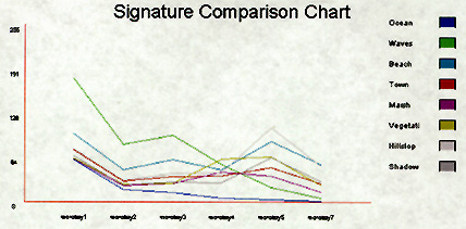
The signature positions at each band are somewhat artificial in that the raw data were not adjusted for relative gains; this affects Bands 1 and 5 in particular. However, it is clear from these plots that most of the signatures are different from one another over the 6 bands used, even though some are close-spaced (nearly coincident) over intervals consisting of several adjacent bands, e.g, all but Waves and Beach between TM1 and TM2. The greatest separability among all classes occurs in Band 5.
IDRISI also has a program that presents pixel information for each signature, recording the number of pixels contributing to the data, and the mean, maximum, minimum, and standard deviation of DN values for each signature. To help you get a deeper feel for the numerical inputs involved in these calculations, we have reproduced a simplified version of these data in the following table:
Table of Band Means and Sample Size for Each Class Training Set
BAND:
1
2
3
4
5
6 (TH)
7
No. of
Pixels
Class
Seawater
57.4
16.0
12.0
5.6
3.4
112.0
1.5
2433
Sediments1
62.2
19.6
13.5
5.6
3.5
112.2
1.6
681
Sediments2
69.8
25.3
18.8
6.3
3.5
112.2
1.5
405
Bay Sediment
59.6
20.2
16.9
6.0
3.4
111.9
1.6
598
Marsh
61.6
22.8
27.2
42.0
37.3
117.9
14.9
861
Waves Surf
189.5
88.0
100.9
56.3
22.3
111.9
6.4
1001
Sand
90.6
41.8
54.2
43.9
86.3
121.3
52.8
812
Urban1
77.9
32.3
39.3
37.5
53.9
123.5
29.6
747
Urban2
68.0
27.0
32.7
36.3
52.9
125.7
27.7
2256
Sun Slope
75.9
31.7
40.8
43.5
107.2
126.5
51.4
5476
Shade Slope
51.8
15.6
13.8
15.6
14.0
109.8
5.6
976
Scrublands
66.0
24.8
29.0
27.5
58.4
114.3
29.4
1085
Grass
67.9
27.6
32.0
49.9
89.2
117.4
39.3
590
Fields
59.9
22.7
22.6
54.5
46.6
115.8
18.3
259
Trees
55.8
19.6
20.2
35.7
42.0
108.8
16.6
2048
Cleared
73.7
30.5
39.2
37.1
88.4
127.9
45.2
309
` <>`__1-22: Examine the signature plots and the table. What can you say about the plots in terms of similarities and differences? Based on numbers in the table, would you predict any notable differences in the signatures for towns; marsh; sunlit hillslopes and shadows? `ANSWER <Sect1_zanswer.html#1-22>`__
We can deduce from this table that most of the signatures have combinations of DN values that allow us to distinguish on from another, depending on the actual standard deviations (not shown). Two classes, Urban 1 and Cleared (Ground), are quite similar in the first four bands but apparently are different enough in Bands 5 and 7 to suppose that they are separable. The range of variations in the thermal Band 6 is much smaller than in other bands, suggesting its limitation as an efficient separator. However, as we will see next, its addition to the Maximum Likelihood Classification increases the spatial homogeneity of some classifications.