Remote Sensing Tutorial Page 1-12a
Almost without exception, the image will be significantly improved if one or more of the functions called Enhancement are applied. Most common of these is contrast stretching. This systematically expands the range of DN values to the full limits determined by byte size in the digital data. For Landsat this is determined by the eight bit mode (28) or 0 to 255 DNs. Examples of types of stretches and the resulting images are shown. Density slicing is also examined.
Contrast Stretching and Density Slicing
We move now to two of the most common image processing routines for improving scene quality. These routines fall into the descriptive category of Image Enhancement or Transformation. We used the first image enhancer, contrast stretching, on most of the TM images we have looked at so far in the previous 11 pages to enhance their pictorial quality . Different stretching options are described next, followed by a brief look at density slicing We will then evaluate the other routine, filtering, shortly.
As we said on page 1-4, contrast stretching, which involves altering the distribution and range of DN values, is usually the first and commonly a vital step applied to image enhancement. Both casual viewers and experts normally conclude from direct observation that modifying the range of light and dark tones (gray levels) in a photo or a computer display is often the singlemost informative and revealing operation performed on the scene. When carried out in a photo darkroom during negative and printing, the process involves shifting the gamma (slope) or film transfer function of the plot of density versus exposure (H-D curve). This is done by changing one or more variables in the photographic process, such as , the type of recording film, paper contrast, developer conditions, etc. Frequently the result is a sharper, more pleasing picture, but certain information may be lost through trade-offs, because gray levels are “overdriven” into states that are too light or too dark.
Contrast stretching by computer processing of digital data (DNs) is a common operation, although we need some user skill in selecting specific techniques and parameters (range limits). The reassignment of DN values is based on the particular stretch algorithm chosen (see below). Values are accessed through a Look-Up Table (LUT).
The fundamental concepts that underlie how and why contrast stretching is carried out are summarized in this diagram:
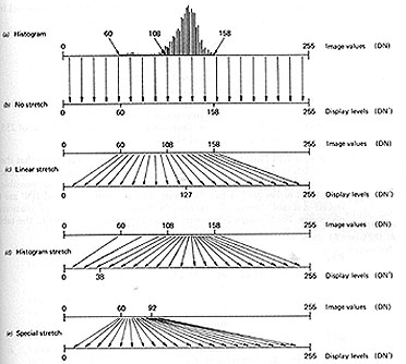
From Lillesand & Kiefer, Remote Sensing and Image Interpretation, 4th Ed., 1999
In the top plot (a), the DN values range from 60 to 158 (out of the limit available of 0 to 255). But below 108 there are few pixels, so the effective range is 108-158. When displayed without any expansion (stretch), as shown in plot b, the range of gray levels is mostly confined to 40 DN values, and the resulting image is of low contrast - rather flat.
In plot c, a linear stretch involves moving the 60 value to 0 and the 158 DN to 255; all intermediate values are moved (stretched) proportionately. This is the standard linear stretch. But no accounting of the pixel frequency distribution, shown in the histogram, is made in this stretch, so that much of the gray level variation is applied to the scarce to absent pixels with low and high DNs, with the resulting image often not having the best contrast rendition. In d, pixel frequency is considered in assigning stretch values. The 108-158 DN range is given a broad stretch to 38 to 255 while the values from DN 107 to 60 are spread differently - this is the histogram-equalization stretch. In the bottom example, e, some specific range, such as the infrequent values between 60 and 92, is independently stretched to bring out contrasty gray levels in those image areas that were not specially enhanced in the other stretch types.
Commonly, the distribution of DNs (gray levels) can be unimodal and may be Gaussian (distributed normally with a zero mean), although skewing is usual. Multimodal distributions (most frequently, bimodal but also polymodal) result if a scene contains two or more dominant classes with distinctly different (often narrow) ranges of reflectance. Upper and lower limits of brightness values typically lie within only a part (30 to 60%) of the total available range. The (few) values falling outside 1 or 2 standard deviations may usually be discarded (histogram trimming) without serious loss of prime data. This trimming allows the new, narrower limits to undergo expansion to the full scale (0-255 for Landsat data).
Linear expansion of DN’s into the full scale (0-255) is a common option. Other stretching functions are available for special purposes. These are mostly nonlinear functions that affect the precise distribution of densities (on film) or gray levels (in monitor image) in different ways, so that some experimentation may be required to optimize results. Commonly used special stretches include:1) Piecewise Linear, 2) Linear with Saturation 3) Logarithmic, 4) Exponential 5) Ramp Cumulative Distribution Function, 6) Probability Distribution Function, and 7) Sinusoidal Linear with Saturation.
Now, to apply these ideas to the Morro Bay TM bands. For Landsat data, the DN range for each band, in the entire scene or a large enough subscene, is calculated and displayed as a histogram (recall the histogram for TM Band 3 of Morro Bay on page 1-1; there is a frequency peak at about DN = 10 and most of the pixels fall between DN 0 and DN 60).

When IDRISI’s standard linear stretch program was applied, this somewhat improved image resulted.
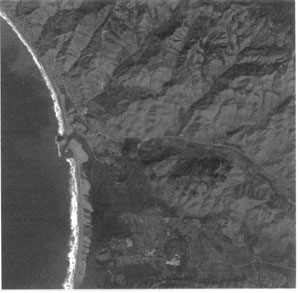
Band 3 image of Morro Bay after a linear stretch.|
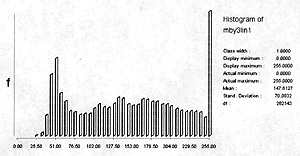

The histogram for this image is polymodal, with a lower limit near 25 and a large number of DN pixels at or near 255. This accounts for the greater scene brightness (light tones).
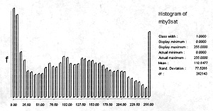

The image appears as a normal and pleasing one, not much different from the others. But, comparing this one with either of the linear-stretched versions shows that real and informative differences did ensue.


The image is similar to the Saturation version. Note that pixel frequencies are spread apart at low DN levels and (closely-spaced) at high intervals.
Let us reiterate. Probably no other image processing procedure or function can yield as much new information or aid the eye in visual interpretation as effectively as stretching. It is the first step, and most useful function, to apply to raw data.
` <>`__1-12: Comments have been made above about the relative quality and information content of each of the stretches displayed. In your opinion, which seems best and is most pleasing to the eye. `ANSWER <Sect1_zanswer.html#1-12>`__
Another straightforward form of enhancement results from the combining (“lumping together”) of DNs of different values within a specified range or interval into a single value. This density slice (also called “level slice”) method works best on single band images. It is especially useful when a given surface feature has a unique and generally narrow set of DN values. The new single value is assigned to some gray level (density) for display in a photo or on the computer monitor (or in an alphanumeric character printout). All other DNs can be assigned another level, usually black. This yields a simple map of the distribution of the combined DNs. If several features each have different (separable) DN values, then several gray level slices may be produced, each mapping the spatial distribution of its corresponding feature. The new sets of slices are commonly assigned different colors in a photo or display.
Version 2.0 of IDRISI FOR WINDOWS unfortunately does not have a simple density slicing routine, so the Morro Bay scene cannot be used here to illustrate this type of enhancement. But below is a good substitute showing two multi-level color slices of a subscene around Harrisburg, PA (this scene will be considered in detail during the “Exam” that you are encouraged to work through at the end of this Section). The sliced subscenes are from MSS Band 6 (vegetation bright) acquired in July 1975:
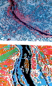
The upper map has four levels or slices. The lavender tends to demarcate a gray level (DN 43 to 48) that associates with urban areas. The lower map (pixels enlarged) covers part of the northern reaches of Harrisburg (the bridge is Interstate 81). Six gray levels (each representing a DN range) have been colorized as follows: Black = (DN) 0-19; Blue = 20-34; Red = 35-44; White = 45-54; Brown = 55-69; Green = 70+. The black pattern is almost entirely tied to water; the blue denotes heavily built up areas; the green marks vegetation; the other colors indicate varying degrees of suburbanization and probably some open areas.