Spatial Filtering
Contents
Just as contrast stretching strives to broaden the image expression of differences in spectral reflectance by manipulating DN values, so spatial filtering is concerned with expanding contrasts locally in the spatial domain. Thus, if in the real world there are boundaries between features on either side of which reflectances (or emissions) are quite different (notable as sharp or abrupt changes in DN value), these boundaries can be emphasized by any one of several computer algorithms (or analog optical filters). The resulting images often are quite distinctive in appearance. Linear features, in particular, such as geologic faults can be made to stand out. The type of filter used, high- or low-pass, depends on the spatial frequency distribution of DN values and on what the user wishes to accentuate.
Spatial Filtering
Another processing procedure falling into the enhancement category that often divulges valuable information of a different nature is spatial filtering. Although less commonly performed, this technique explores the distribution of pixels of varying brightness over an image and, especially detects and sharpens boundary discontinuities. These changes in scene illumination, which are typically gradual rather than abrupt, produce a relation that we express quantitatively as “spatial frequencies”. The spatial frequency is defined as the number of cycles of change in image DN values per unit distance (e.g., 10 cycles/mm) along a particular direction in the image. An image with only one spatial frequency consists of equally spaced stripes (raster lines). For instance, a blank TV screen with the set turned on, has horizontal stripes. This situation corresponds to zero frequency in the horizontal direction and a high spatial frequency in the vertical.
In general, images of practical interest consist of several dominant spatial frequencies. Fine detail in an image involves a larger number of changes per unit distance than the gross image features. The mathematical technique for separating an image into its various spatial frequency components is called Fourier Analysis. After an image is separated into its components (done as a “Fourier Transform”), it is possible to emphasize certain groups (or “bands”) of frequencies relative to others and recombine the spatial frequencies into an enhanced image. Algorithms for this purpose are called “filters” because they suppress (de-emphasize) certain frequencies and pass (emphasize) others. Filters that pass high frequencies and, hence, emphasize fine detail and edges, are called highpass filters. Lowpass filters, which suppress high frequencies, are useful in smoothing an image, and may reduce or eliminate “salt and pepper” noise.
Convolution filtering is a common mathematical method of implementing spatial filters. In this, each pixel value is replaced by the average over a square area centered on that pixel. Square sizes typically are 3 x 3, 5 x 5, or 9 x 9 pixels but other values are acceptable. As applied in lowpass filtering, this tends to reduce deviations from local averages and thus smoothes the image. The difference between the input image and the lowpass image is the highpass-filtered output. Generally, spatially filtered images must be contrast stretched to use the full range of image display. Nevertheless, filtered images tend to appear flat.
Next, we will apply three types of filters to TM Band 2 from Morro Bay. The first that we display is a lowpass (mean) filter product, which tends to generalize the image:
In this example, the scene has been radically modified. The Sobel Edge Enhancement algorithm finds an overabundance of discontinuities but we have chosen this program (using Idrisi) to emphasize the sharp boundaries that can result from applying this mode of enhancement.

` <>`__1-13: Comment further (evaluate) the three filter images shown above in terms of what information you extract visually. Include detrimental aspects. `ANSWER <Sect1_zanswer.html#1-13>`__
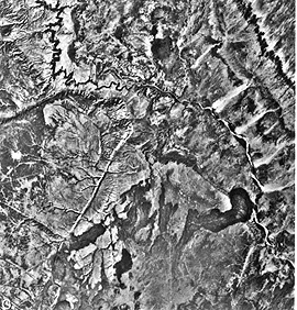
You will note in the answer to this question that the IDRISI filter products leave something to be desired. They can’t really convince one that spatial filtering brings about helpfully different imagery. To assuage that criticism, we are adding (in May 2000) five images extracted from the textbook by Avery and Berlin (Macmillan Publ.; see Overview for reference). The Landsat TM 5 subscene shows a plateau landscape north of Flagstaff, AZ, with both sedimentary rocks and volcanic flows. The first image is just a normal contrast-stretched version.
Flagstaff, AZ on the Colorado Plateau; note volcanic flows.|
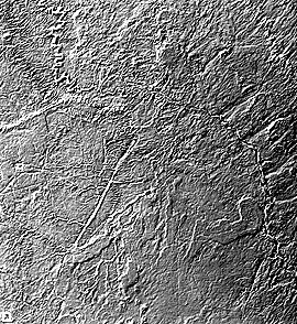
The next view shows this scene as a low bandpass image.
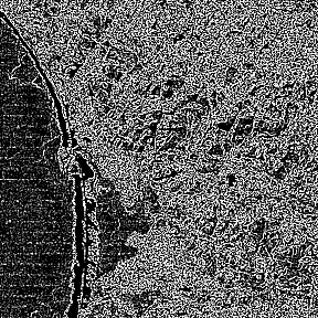
This is followed by a high pass filter image in which the convolution matrix is 11 x 11 pixels. This is made by subtracting the low pass filter image from the original (unstretched) data set. In this instance, the image is a form of edge enhancement.

As the number of pixels in the convolution window is increased, the high frequency components are more sharply defined. That is evident in this image which uses a 51 x 51 pixel matrix.
The last image in this set illustrates directional first differencing, analogous to determining the first derivative which establishes a gradient of spatial change as the filter, with its special algorithm, moves (computer calculational-wise) across the pixel array making up the image. Directional filtering from different directions tends to enhance or disclose linear features that lie preferentially near the perpendicular to the traverse direction. In the image below, the array was moved diagonally across the scene. Note the similarity to the third image above.