False Color Rendition
The page begins with an “aside”, namely, a brief discussion of what has been called “linears” (these will be discussed further in Section 2). The first example of a color composite, made by combining (either photographically or with a computer-processing program) any three bands of images with some choice of color filters, usually blue, green, and red. The single image on this page is that of the customary false color composite made by project a green band image through a blue filter, a red band through green, and the photographic infrared image (in MSS, Bands 6 or 7; in TM, Band 4) through a red filter. Several characteristic color signatures are discussed.
Before leaving this seven-band review, we comment on a peripheral item but one that illustrates a typical danger and misuse of space imagery. Look at any of the images (particularly bands 5 and 7) at two points marked **w**. You should see two thin dark features that are almost straight. These “linears,” as some call them, are common phenomena, observed in satellite images and in aerial- or astronaut-camera photographs. Peruse the rest of the image you chose and you should find more linears (although some are actually sharp boundaries between two features or classes). In the early days of Landsat applications, many geologists reported that the MSS (and, later, TM) sensor was especially adept at highlighting such linear features. They chose to identify a significant fraction of these features as geological in nature, such faults or fracture systems. Maps showing numerous linears of presumed faults or fractures were produced and often published but too frequently without appropriate field checking. When several exacting studies discredited this interpretation of many such features (although some, and sometimes a majority, were verified), this use of Landsat led to widespread skepticism and negative criticism. Today, we know to be careful, and properly use field inspections to verify our work. Incidentally, we haven’t established the nature of the two linears at **w** but one is probably vegetation lining a narrow gully. The fact that the two line up may be a coincidence and does not prove any commonality.
` <>`__1-10: Make a list of other features besides faults and fractures that have linear expressions. `ANSWER <Sect1_zanswer.html#1-10>`__
False Color Rendition
We are now in a position to upgrade our image processing by generating first, some color composite combinations and then, showing two special types of end product - principal components images and classified images.
Let’s start by producing the now-conventional false color composite, made by assigning TM Band 2 (green) to the blue electron gun in the monitor, Band 3 (red) to the green gun, and Band 4 (the near or photographic reflective IR) to the red gun.
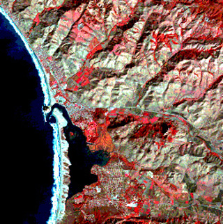
Two color patterns dominate the land classes: reds, depicting vegetation, and medium grayish-browns, found mainly along the bright sun-facing slopes. The ocean and the bay are evinced in deep blues that, near the shore (**a**), become a bit lighter where thicker sediments add reflectance. The breakers are presented in mottled blue and white patterns.
We can place the various expressions of vegetation in several categories based on their specific red tints and in most cases also from the spatial patterns they occupy. The continuous and rather deep red at **g** represents a segment of the forested areas in the Los Padres National Forest near the crest of the Santa Lucia Mountains. Elsewhere, as at **i**, we can attribute thin strings of red or irregular red patches (**j**) to trees and/or scrub vegetation (as at **l**), lining stream channels or scattered as copses and patches along the slopes. In the valleys, bright red areas (at **k** and other points), some rectangular and others more uneven, are primarily examples of field crops, hay meadows, or other types of cultivation. Areas believed to be barren to varying degrees (as at **m** and **o**), have darker gray-brown tones, but may have faint pink overtones implying limited vegetation cover. Where vegetation is sparse and scattered on the hills, particularly where well-illuminated by the sun, the prevailing tan to grayish brown colors imply joint contributions from underlying soils, combined with reflectances from the brown grasses (with much diminished Band 4 input). However, we temper this last statement by the fact that the image produced for this same scene by EOSAT (not reproduced here but examined by the writer) shows more pinks over most of the grassland areas than does this image. At the time of this scene acquisition (mid-November), if winter rains had started early, and had been only moderate to this date, the hills would still be relatively brownish. However, the EOSAT rendition suggests some greening had started.
` <>`__1-11: In the above false color composite, consider a different combination of colors and bands. Make Band 4 = blue; Band 3 = red; Band 2 = green. Describe the general appearance of this new fcc. `ANSWER <Sect1_zanswer.html#1-11>`__
Once again, identify the urban areas from the street patterns. The streets, as well has Highway 1 and other major roadways, have bluish tones, expected because they are especially light-toned in Bands 1 and 2 (assigned here to blue). The mixed tones in Los Osos, with some yellow-brown scattered about, give it a subtly different color signature when compared with Morro Bay. We’ll explain more about this difference when we examine the next color composite. Both town areas contain segments that have red blotches, which correspond to residential sections, park land, or other places where trees or grass grow. The extraction pits (**u**) are very bright, tinged with blue.