The Vegetation Index; Other Vegetation Scenes
Contents
This page considers more examples of practical uses of remote sensing in studying several aspects of vegetation. The first introduces the concept of “Vegetation Index” in which bands sensitive to chlorophyll absorption and cell wall reflectance are treated by simple mathematics (usually ratios of individual bands or of band sums or differences) to accentuate recognition of and variation within types and densities of growing forests, fields, and crops. A now famous example of vegetation changes over growing seasons in the entire African continent, as imaged by the AVHRR sensor on a NOAA satellite, is presented. Other AVHRR examples display NDVI results for Canada, Mexico, and the whole Earth’s landmasses. Another example looks at wheat fields along the Volga River in southern Russia, as seen in Landsat images taken at dates about 3 weeks apart in 1974 and 1975, in which crops in the latter year are greatly reduced in vigor and extent owing to a major drought. A similar situation affected East Africa in 1984 and was monitored by the AVHRR. The final scene includes a Landsat view of the California-Mexican border just above the Gulf of California, in which a striking contrast in number of fields planted and degree of growth results from different crop practices and water uses. Two ASTER scenes covering the same region are also depicted. All these observations, especially at AVHRR scales, are needed as input to integrated data systems that monitor crops at regional and global levels.
The Vegetation Index; Other Vegetation Scenes
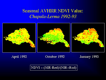
The Landsat and SPOT systems participated in crop control and inventories of various kinds. As stated earlier, Landsat Thematic Mapper (TM) 4 and Multispectral Scanner (MSS) 6 and 7 bands (and SPOT Band 3) are the most sensitive for detecting IR reflectances from plant cells (modified by water content). TM Band 3 and MSS Band 5 (and SPOT Band 2), which measure reflectances in the visible red, provide data on the influence of light-absorbing chlorophyll. Ratio images using these bands help to quantify the amount of vegetation, as biomass, involved in signature responses. For the NOAA series, Bands 2 and 1 of their Advanced Very High Resolution Radiometer (AVHRR) sensor are roughly equivalent to TM Bands 4 and 3 (see Section 14 for a review of metsat systems). The ratio of TM Band 4 to Band 3, MSS Bands 6 or 7 to Band 5, or AVHRR Bands 2 to 1 is a simple approximation of the Vegetation Index (VI). Other VI variants depend on other combinations of these variables. Most commonly used is the Normalized Difference Vegetation Index (NDVI), which is defined as (Near IR band - Red band) divided by (Near IR band + Red band). For TM this is (4 - 3)/(4 + 3); for AVHRR this is (2 - 1)/2 + 1).
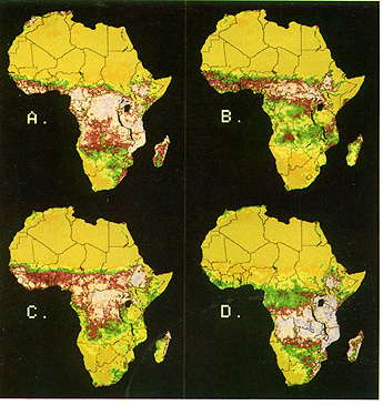
VI distributions for entire continents can be monitored in one view from geostationary satellites such as the meteorological satellite (this is the origin of the common descriptive term, “metsat”). Using AVHRR data (and supporting ground truth) grouped into 21-day periods for eight observing intervals (by NOAA-7) April 1982, through mid-February 1983, J.C. Tucker and his associates at NASA’s Goddard Space Flight Center have produced, using Principal Components Analysis, a general classification of land-cover types for all of Africa. In the class map below medium blue = thickets and bushlands; dark blue = interspersed tropical forests and grasslands; purple = Sudan-type grasslands and woodlands; medium green = semi-arid wooded grasslands and bushlands; dark green = woodlands; yellow = deciduous bushlands and wooded grasslands; orange = semi-deserts to deserts; and red = tropical rainforests and montane forests.
|A Vegetation Index (NDVI) map using two AVHRR bands on NOAA-7 showing the general distribution of various types and degrees of vegetation cover over the entire African continent, as integrated from April 1982 through February 1983. |
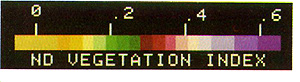
This group and others have continued to apply metsat AVHRR to observe seasonal changes in biomass (“green wave”) over all of Africa, as illustrated below for the following dates: A. April 12-May 2, 1982; B. July 5-25, 1982; C. Sept. 27-Oct. 17, 1982; D. Dec. 20, 1982-Jan. 9, 1983. This has proved invaluable in determining crop shortfalls and drought conditions in Ethiopia and in areas of the Sahel (northern desert regions) during periods in the last decade where starvation was a mass threat. This observational technique has now been applied worldwide.
|
|
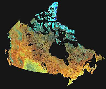
AVHRR data allow monitoring of vegetation over scales ranging from continental, as above, down to regional or up to global. Here is a color mosaic made from Band 1 = blue; Band 2 = green; and NDVI = red for all of Canada. The browns that result indicate the wide extent to which that country is forested.
Much smaller areas can be studied with AVHRR, Landsat, SPOT, and other systems. The next three images, whose information content is given in their titles, cover a large drainage basin in the central Mexican Highlands. The Lerma River flows through the scene into Chapala Lake. This region is south of Guadulajara.
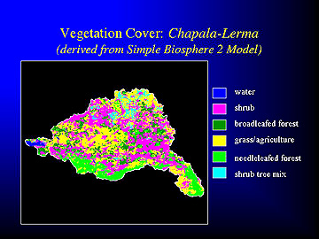
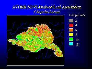
This study, made by Joseph White of Baylor University, can be accessed on the Internet.
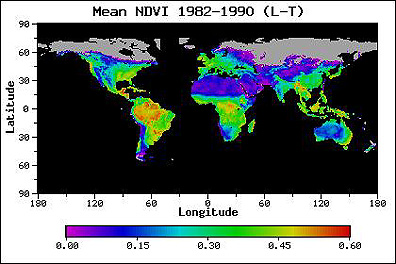
At the other extreme, cumulative AVHRR data allow a plot of mean NDVI distribution on a global basis. This next illustration shows values averaged between 1982 and 1990, using the Los-Tucker model. Note that the highest values are in the Amazon region of South America and the largest low values are in the deserts of North Africa eastward through the Middle East into central Asia.
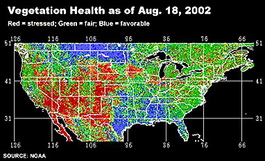
Stressed vegetation can be revealed by NDVI calculations or more directly by other indices. In the summer of 2002, the United States was beset by one of the worse and widespread droughts in decades. (Where the writer [NMS] lives in northeast Pennsylvania, looking out his window on August 21 the lawn is almost totally brown, several trees are losing their leaves, and the foundation plants have wilted; there has been less than 1 inch of rain in the last 6 weeks). (Sparsity of rainfall in early August is discussed at the top of page 14-15. This image is a plot of AVHRR data processed to indicate vegetation stress:
The Volga Wheat Drought; Africa; the Salton Sea, California/Mexico
In the mid-70s, another example of crop failure on a grand scale, but not in Africa, made media headlines. In the Volga and other key wheat growing areas of the former Soviet Union, a severe drought in parts of Russia led to a threatening production shortfall that forced the leaders to seek help from outside wheat markets. They approached the U.S. and Australia governments, in particular, to furnish enough wheat and other grains to forestall possible starvation in several regions. Some critics claimed that the leaders were faking the shortage to take advantage of good prices elsewhere. But, the camera doesn’t lie. Landsat images proved the veracity of the Russian plea for help, as is clearly depicted in this before and after image:
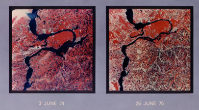
In the 1974 subscene that embraces a large bend in the Volga River, the fields are already in normal crop stages. A year later, and three weeks beyond the 1974 time, when mature crops should have increased the scene redness, instead much of the farmland is fallow (darker grays and tans), confirming the drought claims.
` <>`__3-10: Does the drought appear localized or regional; what is the nature of the red colored area within the great curved bend of the Volga? `ANSWER <Sect3_answers.html#3-10>`__
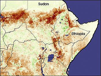
Drought is one of the conditions affecting vegetation that can be sensitively measured by AVHRR NDVI calculations. This next scene covers part of East Africa around the Horn extending from Ethiopia and Somali. The browns indicate abnormally severe stress conditions in the vegetation; yellow is a bit worse than normal; and green correlates with local areas not suffering from the effects of low rainfall.
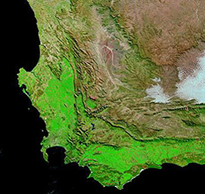
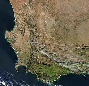
Winter wheat is a staple around Cape Town, South Africa. The next pair of MODIS images were taken exactly 1 year apart on July 21, 2002 and July 21, 2003 during the peak of southern hemisphere growing for this type of wheat crop. The greatly reduced green tones in the 2003 natural color image is a strong indication of poor crops owing to a pronounced drop in southern Africa; also affected are the natural grasslands that abound in this climate.
Dry or desert-like regions do actually have considerable vegetation. Arid country is characterized by grasses and brushland. Here is a IRS scene in the Mojave Desert in which the main land cover types have been classified:
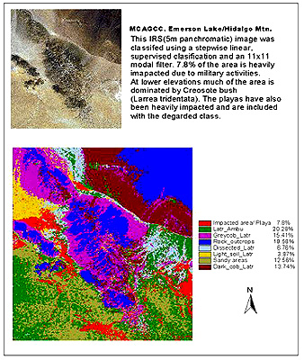
The principal vegetation is the Creosote bush (Larrea Tridentata) which occurs in several settings.
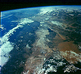
Before leaving this agricultural theme, we want to look into one more example to show one of the most fertile and prolific growing areas in North America. which lies just a hundred miles or so south of the Mojave Desert. This astronaut photo shows much of southern California including the Mojave Desert, the coastal ranges east of San Diego, the Salton Sea and Imperial Valley further east, and a part of Mexico at the northern end of Baja California.
This agricultural region, one of the main producers of winter vegetables in the U.S., extends north and south of the Salton Sea, a saline body of water more than 49 km (30 mi) long, that fills a basin about 82 m. (269 ft) below sea level. This “Sea” was created by an overflow of water from the distant Colorado River (a small segment is visible in the upper right corner) shortly after the beginning of the 20th Century. Floodwaters poured through low dry washes, traveling westward more than 64 km (40 miles) to empty into the lowest part of the Coachella Valley. In this desert climate, that water is slowly evaporating and turning brackish (moderately salty) and is thus not suited for direct irrigation.
The lake-like water at the image bottom is Laguna Salada, which undergoes seasonal drops in level that at times reach a dry state, exposing playa lake beds. East of the Valley are the Chocolate Mountains, part of the Basin and Range system, against whose flanks are conspicuous alluvial fans. The bright strip in the right half of the subscene is the Algodones Dunes field, derived from beach sands left at the surface after an ancient predecessor to the Salton Sea had occupied the Salton Trough, a structural basin between the Coast Ranges (lower left) and the eastern mountains.
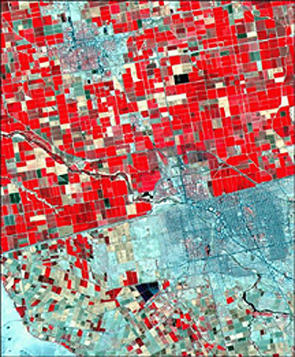
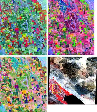
Today, canals from the Colorado River transport water to the sea. The biggest canal in this scene is the prominent All-American canal. Mild winters promote year-round farming (up to three harvests) in the Valley, with cotton, sugar beets, lettuce, and citrus being the main crops. Most fields are in full growth in this April scene, as indicated by the bright, uniform reds. Differences in land use practice and availability of water (no major canals) account for the pronounced decrease in agriculture on the Mexican side. This is visually quite striking when this ASTER close-up of the border land use is examined (El Centro is the town in the U.S.; Mexicali is in Mexico).
The individual fields, which show small differences in the two false color composites above, are hard to pick out in these traditional renditions. In the image below, there are three renditions of the Coachilla Valley farmlands north of the Salton Sea made by different band combinations from the ASTER spectral bands (see page 16-10). These are listed in the caption.
` <>`__3-11: How might a sequence of Landsat or SPOT scenes taken over the months or even years be beneficial to the economic and environmental management of this region? **ANSWER**
Clearly, the differences in expression using different combinations of just these bands suggests the ability to identify, differentiate, and classify the types of crops being grown. The additional bands on ASTER improve this capability, allowing greater accuracy in specifying crop types.
Crop monitoring to control health and estimate harvest output has become a sophisticated system using various multisource data sets. Here is one scheme used by federal agencies and private commodity firms to make predictions or issue warnings about crop damage and other problems.
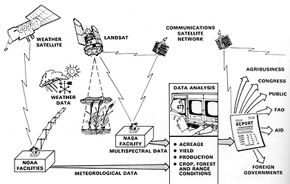
The LACIE, Agristars, and FIFE field experiments were early examples of proof-of-concept. Crop identification can be as high as 90% accurate. The programs require considerable onsite inputs but depend on satellites to provide high resolution multispectral data to extrapolate from the few training sites needed for classification of relatively small areas to maps of the vast regions that are needed to make reliable estimates at country or global scales. We shall consider this theme again in the first part of Section 13.