Field Instruments and Measurements; Data Collection Platforms; GPS
Contents
Measurements with radiometers and spectrometers are carried out primarily to accumulate specific spectral signatures of various materials and features that help to build up a spectral data “bank”. This can be done under controlled laboratory conditions, leading to “representative” signatures for the particular material. Signatures gathered in the field, from portable instruments on tripods or mounted on “cherry pickers”, will include more natural conditions, such as atmospheric effects and solar illumination. Prototype sensors as well as operationally-proven instruments are also flown on aircraft; the data are used either as direct inputs to a remote sensing application or as support for space-mounted sensor studies. Other kinds of useful information about a scene being studied can be monitored by sensors housed on the ground; the data are relayed intermittently or continuously from Data Collection Platforms. The nature of the Global Positioning System (GPS), based on satellite triangulation, is explained.
Field Instruments and Measurements; Data Collection Platforms; GPS
A typical lab spectrometer generates illumination that irradiates a sample mount with diffused light scattered from a metal-plated hemisphere that integrates over an area measured in steradians. Light reflected at an angle from the sample surface collimates as a beam through a hole in the hemisphere. A chopper (rotating signal divider) interrupts the beam by alternately passing and blocking the light that goes to a grating and/or prism, which disperses the radiation into its spectrum. A second beam from a reference source of known and constant intensity reaches the dispersing element during the blocking phase. The dual beam signals then go to a detector that scans them (i.e., moves through the dispersion angles) to measure reflectances (as intensities) as a function of wavelengths. The signals are amplified and then plotted on an X-Y recorder. We display these signals as the ratio of sample reflectance to the reference output, to derive total reflectance (specular and diffuse components). Some instruments can vary the angles of incidence and observation to derive bidirectional reflectance, in which intensities vary with the angles selected (displayed in a series of curves).
Operating the spectrometer in a near vacuum eliminates the effects of absorption bands in the atmosphere. Thus, a series of fixed angle reflectance measurements on some typical rocks from Wyoming (which you first saw on page 2-1), made using a lab (in-doors) spectrometer, appear below for your re-examination. The absorption bands at >2.0 µm and 2.3 µm are associated with mineral constituents and pore water rather than atmospheric gases.
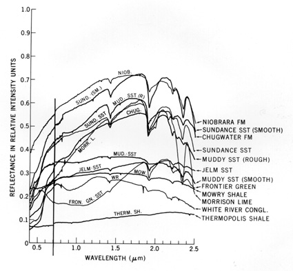
In recent years, the term hyperspectral has come to apply to spectral curves that are either continuous over a broad range, such as the Wyoming group, or consist of a large number of individual narrow-wavelength (high spectral resolution) channels that are so closely spaced that they constitute an almost quasi-continuous spectrum. Until the last decade (see AVIRIS described later in this Section), it was technically very difficult to operate a spectrometer from fast-moving air and space platforms, because the instrument was unable to dwell on a small target (IFOV) long enough to scan the full spectrum. This limitation is the main reason Landsat, SPOT, and other sensor systems have had to use broad wavelength bands that integrate the variations in spectral intervals into single values for the reflectance ranges they represent.
Using spectrometers and related instruments in the field has the advantage of looking at surfaces that contain the mix of components that make up the classes of usual interest (remember the usual constituents in a field crop). We can often obtain spectra for each component and then back away to get the full mix. This collection of component spectra assists in interpreting the mix response. Also, illumination conditions from solar irradiation, plus diffuse skylight and multiple reflections from ground surroundings that can contribute 10% to 25% of the total, during sunny or even overcast conditions, are best in the outdoors.
` <>`__13-10: Suggest three other advantages to acquiring spectral data in the field. `ANSWER <Sect13_answers.html#13-10>`__
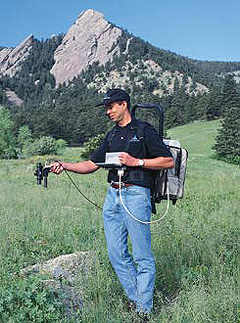
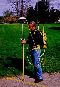
One of the simplest devices is a hand-held two- or three-band radiometer, such as the one held by the writer (NMS) in this illustration:

The instrument has its own portable power source and recording system. The spectral bandwidth is typically 0.05 to 0.10 µm. Common channels are in the green, red, and near-IR. These are especially pertinent to calculating Vegetation Indices (page 3-4).
` <>`__13-11: Specify narrow band wavelengths for vegetation detection using a two or three band radiometer (if you have forgotten what vegetation signatures look like, check Section 3). `ANSWER <Sect13_answers.html#13-11>`__
We can take readings at various look and solar angles, and on different dates and times of year to provide records of spectral variations in the same test areas. These variables can have a pronounced effect on the character of the spectral response, and hence the interpretation of changes, as indicated in this plot of bidirectional reflectances, showing the variation of IR/red-band radiances as a function of view angle and azimuth (compass) direction:
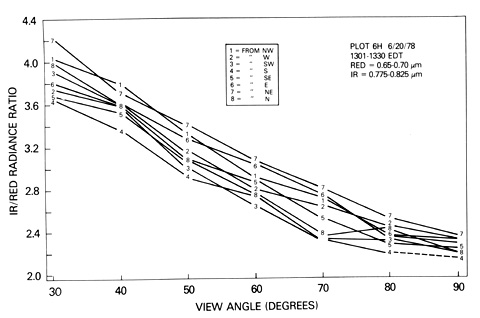
` <>`__13-12: Formulate a generalization about the implications of these curves. `ANSWER <Sect13_answers.html#13-12>`__
In general, spectra of rocks show much less variability, because of bidirectional reflectance effects, than does vegetation. For forests, irregularities in canopy shape, leaf or needle shapes, and species mix can have notable influence on response as a function of viewing and illumination geometry. Portable field spectrometers are now in common use. The next image shows a typical setup for a portable reflectance spectrometer developed by the Jet Propulsion Lab (JPL) in the mid-70s:

For this instrument, an optical head gathers the reflected light and passes it through a filter wheel operating between 0.4 and 2.5 µm onto a cooled detector, made of lead sulphide (PbS). The backpack contains a power source, amplifier, and recording (analog to digital) assembly. After the ground target scan (30 seconds or less) is complete, they quickly repeat the scan on a a flat reference plate made of a high reflectance (near white) material. Sometimes they use a black plate as well, to fix both ends of the reflectance range. Over a brief time span, the scene lighting remains about the same, but over longer periods, changes in clouds, sun angle, etc., cause variations in spectral response. However, they normalize the spectra by dividing the target readings with the reference values. The assumption here is that variations in irradiance over a series of paired readings taken minutes to hours apart cancel, since differences in the illumination conditions affect both target and reference in the same way at each sampling time . For example, if at time 1, at some wavelength, the target reads 30 and the reference 90 and at time 2 they read 20 and 60 (percent), the normalized spectra are both 0.33 (33%) in reflectance units. In the next image, we show field (in situ) reflectance spectra of rocks (1-5) and ponderosa pine (6) acquired by this instrument:

` <>`__13-13: These spectral curves show much less structure (peaks and troughs) and less amplitude (intensity) than the laboratory-produced curves for the Wyoming rocks (above). Explain this difference. `ANSWER <Sect13_answers.html#13-13>`__
JPL engineers, leaders in developing ground truth instruments, developed a portable field emission spectrometer that uses argon-cooled, mercury-cadmium-telluride (HgCdTe) detectors to sense thermal IR responses in the 5 to 15 µm spectral region. In keeping with the trend toward using linear array multispectral systems (e.g., SPOT), instead of scanners with filters (Landsat), some field spectrometers today use a fixed grating that spreads radiation over a range of angles onto array detectors made of indium-gallium-arsenic (InGaAs) alloys capable of more rapid scanning and greater sensitivity. For further insights into field spectrometry, consult the review found on the Home Page prepared by Analytical Spectral Devices, Inc., a company founded by Dr. Alexander Goetz (formerly at JPL), a leader in this field. One of their most versatile field systems is this spectrometer/backpack combo that scans between 0.35 and 2.5 µm, with spectral resolution from 3 nanometers at the low end to 10 nm at the high.
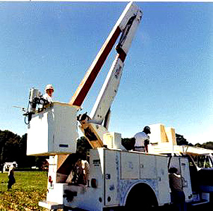
Another approach is to operate a spectrometer from a truck in which we mount the sensor head on a movable cherry picker, as illustrated below. This allows us to vary the Instantaneous Field Of View (IFOV) height, so that we can examine larger surface areas.
Often the user obtains the most valuable supporting data from sensors mounted on aircraft that fly over study areas. In remote sensing programs administered by NASA, investigators specify test sites for acquiring ancillary data or system developers do to test prototype (breadboard) instrument and sensor designs, proposed for future missions. Such research missions help to determine the spectral and spatial resolutions, the signal-to-noise (S/N) response, and the time of day and year that optimize detecting and identifying. We show here part of an earlier fleet of airplanes used for these purposes:
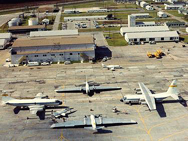
The large plane on the left is a Lockheed Electra that operates up to 7,600 m (25,000 ft). On the right is a C-130, which can be flown at higher altitudes (9200 m or 30,000 ft). The two center planes are RB57F’s that fly up to 18,500 m (60,000 ft). The jet near the hanger has sensors for lower-altitude missions.
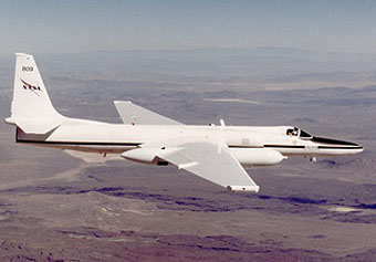
NASA has also used aircraft that fly above the bulk of the stratosphere at altitudes from 60,000 to 70,000 ft. First were two U-2’s decommissioned from the military. In the early 1990’s, NASA contracted with Lockheed, the U-2 builder, to developed a larger version of this aircraft, dubbed the ER-2 (ER stands for Earth Resources). One of these appears below in flight across a desert terrain.
Among the complement of aircraft-mounted sensors are one or more film camera systems (including multiband arrays), multispectral scanners (including those using charge-coupled detectors [CCDs]), thermal-IR scanners (such as the Thermal IR Multispectral Scanner [TIMS], see page 9-7), microwave sensors (including radiometers and scatterometers, and multiband radar), and special request equipment not routinely flown.
At the other extreme, we often need to collect continuous data on the ground at widely separated stations or over extended time periods, often in inaccessible areas. Costs from repeat trips and other factors may preclude sending field parties after initial visits. With such requirements, we set up automated, remote-sensing, sampling sites, at which we measure several defining properties constantly or at fixed intervals.
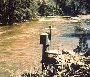
To accomplish this during the Landsat program, NASA and other organizations, including Principal Investigators in research and verification programs, deployed Data Collection Platforms (DCPs) to measure certain properties on site, coding the results and transmitting these by radio whenever Landsat or some other satellite was in line of sight, and then relayed the data to appropriate ground stations for processing. Typical remote field measurements include: 1) stream heights and velocities; 2) silt loads; 3) snow pack densities; 4) meteorologic parameters; 5) point source pollution; 6) seismic disturbances, and 7) surface tilt on volcano slopes. We now commonly use networks of remote stations in the U.S. and other countries, such as this example of a stream hydrograph and its transmitter:
` <>`__13-14: Cite three other plausible uses for DCPs - these need not be directly pertinent to Landsat-type observations. `ANSWER <Sect13_answers.html#13-14>`__
In performing field studies and measurements, it often proves difficult to know exactly where you are. In the early Landsat days, finding one’s self at a site where something in the imagery is being checked out was generally an approximation at best. With the advent and full implementation of the Dept. of Defense (DOD) Global Positioning System (GPS) program in the late 1960s, a new means was developed to locate a point on the Earth’s surface to an accuracy within 70 m or less, and to just a few meters when special adjustments were made.
When all the needed satellites were launched over an extended period, this configuration was achieved:
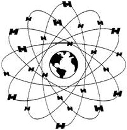
There are six near circular orbits around Earth, each 60° from the orbits on either side. The orbital altitude is approximately 11000 nautical miles (20,200 km). Each orbital path contains 4 properly spaced satellites, for a total of 24 (currently 27; 3 are spares). Each satellite makes two complete orbits in a day - passing an area of the globe once every 12 hours. The orbital mechanics are organized so that from any point on Earth a minimum of three, and usually 4, satellites from several orbital planes are in positions where they can read radio signals from a ground transmitter/receiver.
Communication with a GPS satellite by radio allows the ground-satellite transit to be a simple ranging action. That is, knowing the speed of radio waves (EM, the speed of light), the system on the ground measures the precise delay time in receiving the sent signal. Adjustments for various factors improves the quality of location. Since the particular satellite’s position is also known, the length of the signal vector is established. This in effect results in a virtual sphere of space defined by the vector length. That signal is also sent simultaneously to two other “in view” satellites, yielding two more vectors (radii) and two more spheres. Location now becomes a straightforward problem in triangulation. The intersection of the three spheres produces two common points, one of which makes sense - and is selected as the appropriate location - if the user has a good idea where he/she is. The returned signal from a fourth satellite helps to reduce or eliminate clock errors (related to the atomic clocks onboard each satellite which are not exactly synchronized. A method called Differential GPS, which uses a fixed base station receiver elsewhere to make further corrections can improve accuracy of location to 3 meters (at present, available only for military operations).
Presently, the NAVSTAR (Navigational Satellite Timing and Ranging) system is fully operational. Location or geographic position is reported either in latitude-longitude (down to seconds) or in Universal Transverse Mercator (UTM) coordinates. Survey teams supporting ground truth measurements use setups similar to this:
GPS is finding its way into wide civilian use. For example hunters in a game forest may wish to know where they are (lost?). The instrument below is hand-held; GPS systems are also being installed in automobiles so that any driver can almost automatically establish the car’s location and can also use a complementary system that determines the best routing to destination.

This closes the first part of this Section. The next three pages explore the meaning and uses behind the “multi” concept.
Primary Author: Nicholas M. Short, Sr. email: nmshort@nationi.net