
Road traffic management
In recent years, the application of GIS has paid more attention to traffic , and a special traffic geographic information system (GIS-T) has been formed to meet the requirements of road traffic management. The following sections introduce the specific application of GIS in highway.
Road profile design
Road profile design is an important link in highway design and a step to determine the final direction of highway. In road profile design, a variety of spatial data should be synthetically analyzed, including large-scale land use maps, topographic maps and existing road networks.
Data collected from various aspects are merged into GIS databases, constrained polygons are constructed, and areas to be avoided by highways are determined. Usually these polygons can be divided into three levels:
The first level constraints must be avoided or minimized;
The second constraint is to avoid or minimize it as far as possible;
The third level constraint can be avoided or minimized.
Weights can be used to represent different levels of constraints as needed and displayed separately on maps so that designers can avoid these areas as much as possible when designing routes. Then each experimental line is input into GIS, and the buffer analysis is used to get the polygon of the road profile, and the overlay analysis is carried out with the constraint polygon. The total area of the intersection of the road profile and each polygon are calculated and multiplied by the weight. The total impact weighted area (TIWA) of the constraint influence of the test line is obtained, which is used to compare the design of these lines.
After calculating TIWA, the detailed design of the alignment can be carried out according to DEM. The main operation is to get the road cross-section according to DEM, and then optimize the filling and excavation to get the final road profile design results.
Road management
Attributes involved in road management
In highway management, it is usually necessary to classify roads according to their categories, number of lanes and types of pavement. Its management attributes include:
Highway attributes: Road network marking, road marking, section marking, reference points, etc.;
Geometric attributes: Pavement width, road direction, number of lanes, slope, etc;
Facility attributes: Central isolation belt and isolators, rails, bridges, traffic signs, street lights, traffic volume calculators;
Public facilities: Toll stations, intersections, culverts, traffic management stations, etc;
Attributes of building materials: Surface, overburden, base, roadbed;
Statistical attributes of road use: Traffic volume, average daily flow, accidents, vehicle weight statistics, vehicle type statistics, route requirements;
Acceptance record attributes: Strength, roughness, obstacles, pavement damage, speed limit section, speed survey;
Contract attributes: Budget, expenses, plans, dates, etc;
Maintenance engineering attributes: Project category, budget, cost, quantity, date.
These attributes are correlated with road network by linear positioning method. Generally, there are milestone method and control section method for linear positioning. The former uses road names and mileage points on highways to determine the location of objects. The latter divides highways into connected and different length control sections, each section has a code, and its attributes are identical (Table 2).
Table 14-2: Recording attributes using control segment method
Control Segment |
Surface |
Lane Numbers |
State |
Starting Point |
Ending Point |
|---|---|---|---|---|---|
CS1 |
Gravel |
2 |
bad |
||
CS2 |
asphalt |
4 |
good |
30.08 |
30.16 |
CS3 |
asphalt |
2 |
fair |
30.16 |
30.2 |
CS4 |
asphalt |
2 |
good |
Dynamic segmentation
One of the characteristics of traffic model is that many linear objects overlap on the same road network, such as speed limit section, and public transport lines overlap with the road network. This makes it difficult for GIS to apply to traffic. Dynamic Segmentation method solves this problem.
Dynamic segmentation is to record the distance between the starting and ending points of each attribute of the road and the origin of the road in the database. It does not really cut off the road and store it. It is suitable for dynamic analysis and dynamic segmentation as its name suggests.
After dynamic segmentation, a segment is a part of the line or arc between two intersections on the road network. The length of the segment is expressed by its proportion to the line, and it has a unique identification code. In the GIS database, the section is attached to the road network data and has no coordinates. Because dynamic segmentation is used to manage all kinds of road attributes and their distribution in one layer and linear positioning method is adopted, it is easy to realize overlapping query and analysis of all kinds of “points and lines”, such as:
Traffic flow >800,000 and road conditions = “good” and road grading = “Dart”
Analysis of flow and path
Road network topology
The representation of a road network can emphasize its “geometry” or “topology”. In road design, it is necessary to use its geometric representation, while network analysis focuses on the topological relationship (Fig. 14-6).

Figure 14-6: Two Expressions of Road Network
In the traffic network, the intersection point is a topological intersection between the most lines, that is, the vehicle can turn at the intersection of roads. However, the use of planar graph in GIS and some road relationships need to be correctly expressed in three-dimensional space, such as overpasses. In fact the roads do not intersect directly, but it is an intersection point on the plane graph. However, it shows as a intersection point, which needs to be judged in application, distinguishing between topological intersection point and non-topological intersection point, in order to prevent erroneous network analysis results.
Data Structure for Road Network Analysis
When analyzing road network, we can only pay attention to its topological data representation. Its data structure and related algorithms can adopt the mature ‘graph’ data structure. One of the simplest ways is ‘connected matrix’, which records the connection between nodes (Fig. 14-7).
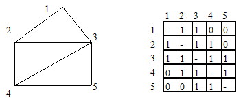
Figure 14-7: Network Connectivity Matrix
In a connected matrix, the value of a cell is 1, which means that two nodes are directly connected, and vice versa, which means that they are not directly connected. Such a connected matrix can be used for connectivity and accessibility analysis. The value of each cell in the matrix can also be the distance between nodes, and the distance between nodes that are not directly connected can be expressed by infinity. The shortest path can be searched by using this matrix. Without considering the directionality of the connection, the graph is undirected, and the connection matrix is symmetric matrix. In urban road traffic, there is often a “one-way line” situation, the connection is directional, so the matrix is asymmetric.
In urban traffic applications, there will be ‘no left turn’ or even ‘no right turn’. At this time, in addition to the connectivity matrix, we need to record the connectivity attributes of each node, which is the intersection, it can also be realized by the connectivity matrix (Fig. 14-8).
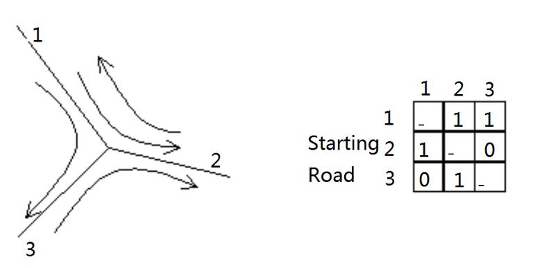
Figure 14-8: Turning and road connectivity matrix of intersections, where the second and third roads are forbidden to turn left
In practical network analysis, it is necessary to make use of the connection matrix of nodes and the connection matrix of roads at nodes.
Specific applications and related models of traffic and network analysis
Traffic flow and network analysis are generally used in urban traffic to provide scientific decision, which support for urban traffic management and road planning. Among them, there are four main models as follows:
Based on the land use patterns of Traffic Analysis Zone (TAZ) and other socio-economic data, the traffic generated and attracted by each region is estimated. For example, residential areas generate travel while commercial areas attract travel.
According to the results of trip generation analysis, the traffic volume between different regions is determined.
The traffic volume calculation is allocated to the vehicles and the traffic volume is calculated.
According to the capacity and speed of the traffic line, the traffic flow is allocated to each road.
The four models mentioned above include statistical analysis operations which are not supported by many traditional GIS tools and specific economic and geographical models. When they are implemented, they can be operated in GIS, and the results can be exported to other systems for professional model calculation.
