
Buffer analysis
Proximity describes the extent to which two objects in geospatial space are close together, and its determination is an important means of spatial analysis. The land along the river or along the river has its unique importance, the service radius of public facilities (shopping, post office, bank, hospital, station, school, etc.), the relocation caused by the construction of large reservoirs, railways, highways and shipping rivers, the importance of economic development through the region is a problem of proximity. Buffer analysis is one of the spatial analysis tools for solving proximity problems.
The so-called buffer zone is an area of influence or service scope of a geospatial target. From a mathematical point of view, the basic idea of buffer analysis is to give a spatial object or set, determine their neighborhood, and the size of the neighborhood is determined by the neighborhood radius R. Therefore the buffer of the object Oiis defined as:
That is, the buffer with the radius R of the object Oi is a set of all points where the distance d from Oiis smaller than R. d is generally the minimum Euclidean distance, but can be other defined distances. For object collection
The buffer whose radius is R is the union of each object buffer, that is:
Figure 8-6 is a buffer example of point object, line object, face object and object set.
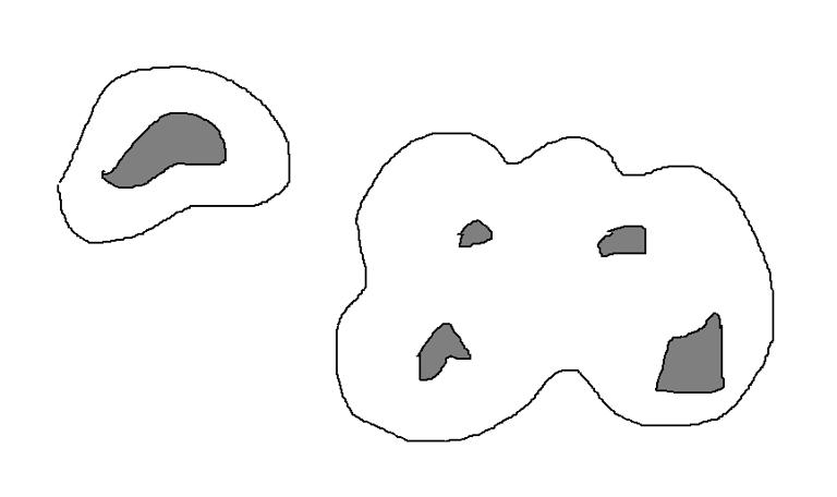
Figure 8-6: Buffers for points, lines and polygons
There are also some special forms of buffers, such as point objects have triangles, rectangles and circles, etc., for line objects, there are bilateral symmetry, double-sided asymmetry or one-sided buffer, and there are inner and outer buffers for the surface object. These buffers are suitable for different application requirements, although the form is special, but the basic principle is the same.
The basic problem of buffer calculation is the two-line problem. There are many other names for double-line problems, such as graph coarsening, widening, center line expansion, etc. They all refer to the same operation.
1) Angle line method
The simplest method for the two-line problem is the angular bisector method (simple parallel line method). At the beginning and end of the axis, the vertical line of the axis is made and the starting and ending points of the left and right side lines are cut out according to the buffer radius R; at other turning points of the axis, the corresponding vertices of the buffer zone are generated by the intersection points of two parallel lines whose distance from the front and back edges to the axis is R. As shown in Figure 8-7.
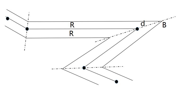
Figure 8-7: Angular bisector method
The disadvantage of the angular bisector method is that it is difficult to ensure the equiwidth of the two lines to the maximum extent, especially when the corner of the convex side becomes sharper, it will be far from the vertex of the axis. According to the figure above, the distance can be expressed by the following formula:
When the buffer radius remains unchanged, D increases with the decrease of the tension angle B, resulting in the destruction of the width between the two lines at the sharp corner.
Therefore, in order to overcome the shortcomings of the angular bisector method, it is necessary to have a corresponding supplementary discriminant scheme to correct the abnormal situation. However, due to the numerous anomalies, the correction measures are complicated.
2) Convex Arc Method
At the beginning and end of the axis, the vertical line of the axis is made and the starting and ending points of the left and right side lines are cut off according to the double lines and buffer radius, at other turning points of the axis, the convexity and concavity of the point are judged first, and the convex side is closed by circular arc, while at the concave side, the corresponding vertices are generated by the intersection points of the two adjacent parallel lines. In this way, the outer corner is connected by an arc, the inner corner is directly connected, and the end of the line segment is closed by a semi-circle, as shown in Figure 8-8.
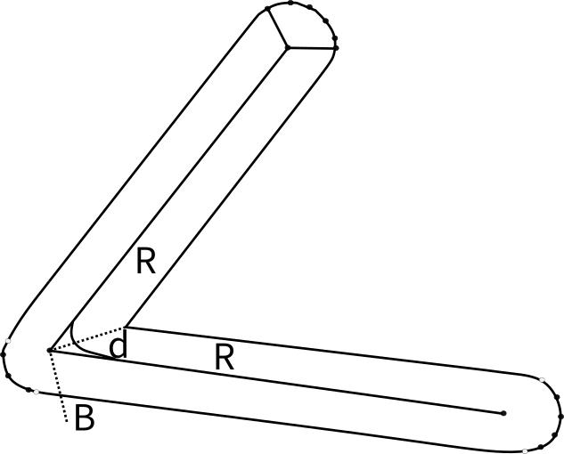
Figure 8-8: Convex Arc Method
Parallel edges on concave sides intersect on angular bisectors. The distance between intersection points and corresponding vertices is similar to the angular bisector method.
This method guarantees the equal width of parallel curves to the greatest extent and avoids many abnormal situations of angular bisector method.
A very important part of the algorithm is the automatic judgment of the eccentricity of the vertices. This problem can be transformed into a cross product of two vectors:The two adjacent line segments are treated as two vectors, and the direction is taken in the direction of the coordinate point sequence. If the previous vector is counterclockwise when sweeping to the second vector at the minimum angle, it is a convex vertex, and vice versa. The specific algorithm process is as follows:
According to vector algebra, vector AB and BC can be expressed by the coordinate difference of their endpoints (9-9):
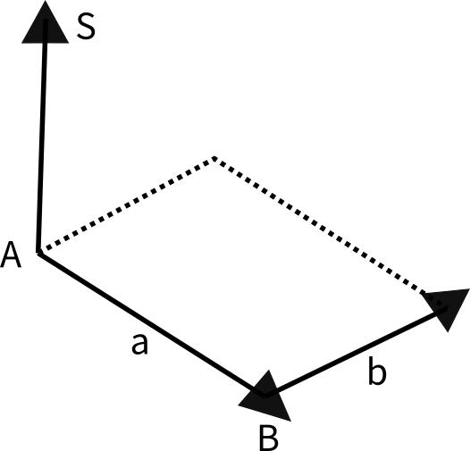
Figure 8-9: Judge vector arrangement with vector cross multiplication
The cross product of vector algebra follows the right hand rule, that is, when ABC is counterclockwise, S is positive, otherwise it is negative.
If S > 0, the ABC is counterclockwise and the vertex is convex.
If S < 0, ABC is clockwise and its vertex is concave.
If S = 0, the ABC points are collinear.
For simple cases, a buffer is a simple polygon, but it is much more complex when calculating buffers for objects with complex shapes or multiple sets of objects. In order to adapt the buffer algorithm to a more general situation, it is necessary to deal with the situation of self-intersection of edges. Several self-intersecting polygons will be generated when the bending space of the axis does not allow the two-line edges to pass through without pressure. Figure 8-10 shows an example of self-intersection of buffer edges.
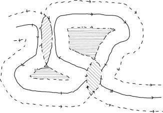
Figure 8-10: Buffer boundary intersection
Self-intersecting polygons can be divided into two cases: Island polygons and overlapping polygons. Island polygon is an effective part of buffer boundary; overlapping polygon is not an effective component of buffer boundary and does not participate in the final reconstruction of buffer boundary. For the automatic identification method of island polygon and overlapping polygon, the axis coordinate point order is defined as its direction, the buffer double line is divided into left and right edge lines, and the discrimination situation of left and right edge line self-intersecting polygon is symmetrical. For the left side line, the island self-intersecting polygon is counterclockwise, the overlapping self-intersecting polygon is clockwise; for the right side line, the island polygon is clockwise, and the overlapping polygon is counterclockwise.
When there are islands and overlapping self-intersecting polygons, the final calculated edges are divided into external edges and several islands. For buffer edge drawing, only peripheral edge and island contour can be drawn. For buffer retrieval, after searching the polygons formed by the outer lines, the results of searching all island polygons should be deducted.
Buffer analysis can also be used for buffer analysis, commonly referred to as shifting or spreading.In fact, the process of moving or diffusing is to simulate the action of the main body on the adjacent object, under the action of the main body, the object moves on a resistance surface, and the farther away from the main body, the weaker the action force is. For example, terrain, obstacles and air can be used as resistance surface, and noise source is the main body. The moving of noise on the resistance surface after leaving the main body can be calculated by the method of shift or diffusion, and the noise intensity of each grid unit in a certain range can be obtained.
