The Birth, Life and Death of Stars
The Birth, Life and Death of Stars
We concentrate on this page on the inception, evolution, and demise of individual stars. A helpful Web Site that supplements the content of this page has been put online by Prof. Nick Strobel of Bakersfield College. Also recommended are the University of Oregon site cited in the Preface (especially relevant are Lectures 15-18, and 20) and a site prepared in outline form by astronomers at University of Georgia.
Before reading the next two pages, it may be profitable for you to get an overview of Star formation by reading a specific page from the above-cited Oregon lectures.
The number of stars in the Universe must be incredibly huge - a good guess is 100 billion galaxies each containing 100 billion stars or (10:sup:11 times 1011, which calculates as 1022 (an independent estimate using other means states the value as 7 x 10²² stars). Yet on a very clear night in dry air, one sees at any one location, without using a telescope or binoculars, about 2500 “star” points within the Milky Way in the northern hemisphere and a similar number in the southern hemisphere. (With a very few exceptions, individual stars outside the M.W. cannot be seen by eye). When viewed from all terrestrial vantage points that number approaches 8400. Some of the of these are distant galaxies, so far away that the unaided eye can discern only an apparent single light source. Many of the brightest stars are generally those closest to the Sun (around 1 to 100 light years away). Only when powerful telescopes are used does the astronomer realize by estimate or extrapolation that billions of galaxies exist; by inference we deduce that these probably contain stars in numbers similar to those that can be roughly counted in the Milky Way (in many tens of billions).
We begin this concentration on stars with something that is itself not truly a scientific topic but which remains useful to astronomers as a convenient “Sky Map”. Such maps contain the Constellations - patterns of certain visible stars (a few were actually galaxies but this was not known at the time) that the ancients imaginatively discerned in looking at individual stars within narrow patches of the celestial hemisphere which seemed to be distinctive and readily recognized. These arrangements were given fanciful names, of gods, animals, and other descriptors from their everyday experiences. This began with the Babylonians in Mesopotamia, and the system was expanded to 88 named constellations by the Greeks and Romans some 2000 years ago. (Psychics and Fortune Tellers have used constellations as “signs” and for horoscopes for several millenia.) This next pair of illustrations (source StarNames) shows some of the major constellations in the northern hemisphere, plotted in two half circle fields:
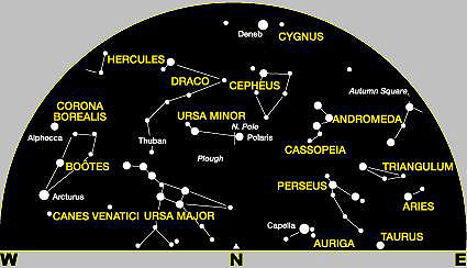
To the ancients, the stars were all equidistant on the “celestial sphere” and varied only in brightness. Modern astronomers now know that individual stars/galaxies in the light points that make up the constellation pattern are actually located at various distances from Earth, which together with diifferences in size account for their different brightnesses. Most of the defining stars in a constellation are located in our galaxy, the Milky Way.
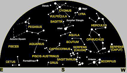
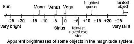
Astronomers often cite individual constellations as a reference framework in specifying the location in the celestial sphere of some stellar or galactic feature or phenomenon on which they are reporting. However, they need to give some specific hemisphere coordinates, either in terms of azimuth, altitude (along a meridian) and hour time, or in another system, the declination and right azimuth. The position of any star as seen on some specific night will vary with the hour, time of year, and geographic location of the observer. Thus, the movement of the Earth around its axis causes the stars during a night’s observation to follow arcuate (circles) paths around a part of the sky where the celestial pole is located (close to the North Star pointed to by two stars in the Big Dipper [Ursa Major]). The groups of constellations also shift with the seasons and with the place on Earth where the star-gazer is positioned (different constellations are seen by those in the Southern Hemisphere of the Earth than those in the Northern Hemisphere [lookers at the Equator will see some of the constellations visible in each Hemisphere]). More about the constellations can be found at the Star Charts and Star Map Internet sites. For the second site, after it appears scroll down until you see in a sentence an underlined phrase called “northern hemisphere constellations”, an example of the usual format of such maps (this one is valid for December). This next map, also from StarNames, shows the same look direction (to the North), as the first map above, but is a Winter view (compare and locate equivalent constellations; but now several have disappeared and new ones have appeared).
Interesting, but back to Science. The standard model for a star is, of course, our Sun. The Sun is typical of most stars; as we shall note shortly, these stellar bodies vary from about 0.1 to 100 times the mass contained in the Sun. Without a telescope, under exceptional viewing conditions (using binoculars), about 9000 individual stars can be seen in the wide celestial band that is the central disc of the Milky Way (M.W.) galaxy. Others elsewhere in the celestial hemisphere make up about 2000 points of stellar light can be seen (in clear air, away from urban light contamination) by the naked eye. Some are nearby within our galaxy and are not particularly large, while others are mostly stars of the Giant/Supergiant types in the halo (see below) around the Milky Way. Still others are galaxies that lie in intergalactic space beyond the Milky Way but mostly within a billion light years from Earth. Telescopes can resolve countless more stars in the M.W., can recognize millions of galaxies, and can pick out some individual stars in nearby galaxies.
A degree of luminosity of an object in the sky (galaxy; star; glowing clouds; planet) can be represented by its apparent magnitude - a measure of how bright it actually appears as seen by the telescope or other measuring device. This magnitude is a function of 1) the intrinsic brightness which varies as a function of size, mass, and spectral type (related to star’s surface temperature)and 2) its distance from Earth. (Magnitude as applied to a galaxy, which seldom shows many individual stars unless they are close [generally less than a billion years away], is an integrated value for the unresolved composite of glowing stars and gases within it.) The brightness of a star can be measured photometrically (at some arbitrary wavelength range) and assigned a luminosity L (radiant flux). For two stars (a and b) whose luminosities have been determined, this relationship holds:
La/L:sub:b = (2.512):sup:m:sub:`b - ma`
from which can be derived:
mb - ma = 2.5 log(La/L:sub:b)
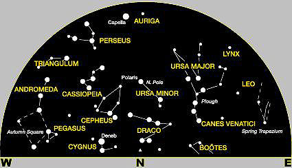
To establish a numerical scale, some reference star(s) must be assigned an arbitrary value. Initially, the star chosen, Polaris, was rated at +2.0 but when it was later found to be a variable star, others were selected to be the 0 reference value for m. The magnitude scale ranges from -m (very bright) to +m (increasingly faint) values. The more positive the number, the fainter is the object (planet; star; galaxy); very distant galaxies, even though these may be extremely luminous, could have large positive apparent magnitudes because of the 1/r2 decrease in brightness with increasing distance. The Sun has the value - 26.5; the full Moon is -12.5; Venus is -4.4; the naked eye can see stars brighter than + 7; Pluto has a magnitude of +15; Earth-based telescopes can pick out stars visually with magnitudes down to ~+ 20 (faintest) and with CCD integrators to about +28, and the HST to about +30. Thus, the trend in these values is from decreasing negativity to increasing positivity as the objects get ever less luminous as observed through a telescope. Each change in magnitude by 1 unit represents an increase/decrease in apparent brightness of 2.512; a jump of 3 units towards decreasing luminosity, say from magnitude +4 to +7, results in a (2.512):sup:3 = 15.87 decrease in brightness (the formula for this is derivable from the above equations, such that the ratio of luminosities is given by this expression: 10(0.4)(m:sub:`b - ma)`. Below is a simple linear graph that shows various astronomical objects plotted on the apparent magnitude scale:
From Nick Strobel’s Astronomy Notes.
Absolute magnitude (M) is the apparent magnitude (m) a star would have if it were relocated to a standard distance from Earth. Apparent magnitude can be converted to absolute magnitude by calculating what the star’s or galaxy’s luminosity would appear to be if it were conceived as being moved to a reference distance of 10 parsecs (10 x 3.26 light years) from Earth. The formula for this is:
M = m + 5 - 5log10r,
where r is the actual distance (in parsecs) of the star from Earth. Both positive and negative values for M are possible. The procedure envisions all stars of varying intrinsic brightnesses and at varying distances from Earth throughout the Cosmos as having been arbitrarily relocated at a single common distance away from the Earth.
Both luminosity and magnitude are related to a star’s mass (which is best determined by applying Newton’s Laws of motion to binary stars [a pair; see below for a discussion of binaries]). The graph below, made from astrometric data in which mass is determined by gravitational effects, expresses this relationship; in the plot both mass and luminosity are referenced to the Sun (note that the numbers are plotted in logarithmic units on both axes):
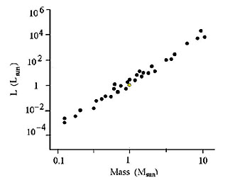
There is a relationship between absolute magnitude (here given by L for luminosity) and mass (given by the conventional letter M; which accounts for replacing the absolute magnitude M with L). Here is one expression:
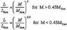
In the above, both L and M for a given star are ratioed to the values determined for the Sun. Note the two different power exponents. It seems that some stars obey a fourth power, others a 3, and a few are just the square of the mass. The most general expression in use is given as L = M3.5. There are relatively few stars with mass greater 50 times the Sun. Very rarely, we can find a star approaching 100s solar mass, but these are so short-lived that nearly all created before the last million years have exploded, with their mass being highly dispersed, and thus ceasing to send detectable radiation.
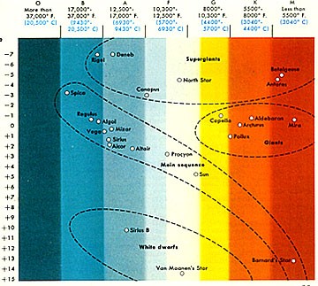
If the Sun were envisioned as displaced outward to a distance of 32.6 l.y., its apparent magnitude as seen from Earth would be -26.5; its absolute magnitude would be changed to +4.85. A quasar, which is commonly brighter than a galaxy, has an absolute brightness of - 27 (note that in the absolute scale increasingly negative values denote increasing intrinsic brightness). The illustration below gives the absolute magnitudes (vertical axis) as a function of temperature (horizontal axis) for a number of stars with popular names; note the similarity of the color bars (which express the visual colors of the stars as seen through a telescope) to the brightness range - this is essentially a preview version of the standard H-D diagram, shown and discussed on this page beginning twelve figures below this, which serves as a plot of the different types of stars and an inferred history of a star of given size (mass):
One classification of stars is that of setting up categories of star types (see below) in a series of decreasing sizes and luminosities. These are the 7 Luminosity/Type Classes: Ia, Ib: Extreme Supergiants; II: Supergiants (Betelgeuse); III: Giants (Antares); IV: Subgiants; V: Dwarfs (Sun): VI: Subdwarfs (metal poor); VII: White Dwarfs (burned out stars). The oddity in this classification is the omission of a category of “Normal”; a star is either a Giant or a Dwarf. Another classification is based on density. Starting with the least dense and progressing to the most dense (massive), this is the sequence: Supergiant; Red Giant; Main Sequence; Brown Dwarf; White Dwarf; Neutron Star; and Black Hole. Each of the above bold-faced types are described in some detail on this two-part page.
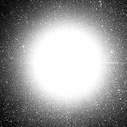
The brightest star in the northern hemisphere of the sky is Sirius, an A type star (see the H-R plots below and accompanying paragraphs which explain the letter designation of stars) of apparent magnitude -1.47 that lies 8.7 light years away. Here is how it appears through a telescope:

Closest to the Sun is an M type star (faint), Proxima Centauri, being 4.2 light years away. Just slightly farther away is Alpha Centauri, a G type star that is the third brightest in the heavens (visible in southern hemisphere). Here is a telescope view of Alpha Centauri:
The map below is a plot of the distances from Earth (circle is 13.1 light years in radius) of the 25 nearest individual or binary stars or local clusters in our region of the Milky Way Galaxy:
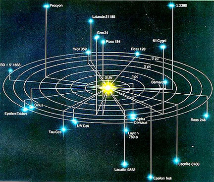
Information Bonus: Just beyond this limit is the star Vega (27 light years away). It has two claims to fame: 1) it alternates with Polaris as the North Star used in navigation; the Earth’s precession brings Vega into this position every 11000 years, and 2) It was the nearby star used as the host for an extraterrestrial civiliation in Carl Sagan’s extraordinary science fiction novel “Contact” (later made into the movie of the same named “starring” Jodie Foster); contact was made with a planet near Vega as a signal picked up by the Socorro, NM radio telescope array - as initially interpreted that signal consisted of a string of prime numbers (those divisible only by themselves and 1).
Referring to the above, the following is extracted verbatim from the caption accompanying this image that was displayed on the Astronomy Picture of the Day Website for February 17, 2002: What surrounds the Sun in this neck of the Milky Way Galaxy? Our current best guess is depicted in the above map of the surrounding 1500 light years constructed from various observations and deductions. Currently, the Sun is passing through a Local Interstellar Cloud (LIC), shown in violet, which is flowing away from the Scorpius-Centaurus Association of young stars. The LIC resides in a low-density hole in the interstellar medium (ISM) called the Local Bubble, shown in black. Nearby, high-density molecular clouds including the Aquila Rift surround star forming regions, each shown in orange. The Gum Nebula, shown in green, is a region of hot ionized hydrogen gas. Inside the Gum Nebula is the Vela Supernova Remnant, shown in pink, which is expanding to create fragmented shells of material like the LIC. Future observations should help astronomers discern more about the local Galactic Neighborhood and how it might have affected Earth’s past climate.
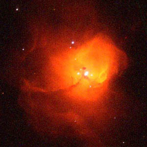
The largest star so far measured in the Milky Way is Mu Cephi (in the galactic cloud IC1396), seen as the orange disc (also called Herschel’s Garnet star) near top center of this HST image. Located about 1800 light years from Earth, it is almost 2500 times the diameter of the Sun.
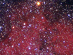
This is an example of a rare type of star known as a hypergiant (see next page). Another even bigger star (2800 times the solar diameter; 2.4 billion miles) is Epsilon Aurigae (in the constellation Auriga, the Charioteer), but residing in the Milky Way about 3300 light years from Earth. This star, also known as Al Maaz (Arabic for he-goat) and visible to the naked eye) is considered by many astronomers to be the “strangest” star in the firmament. Every 27 years this star (magnitude 3.2) undergoes a diminishing of brightness (about 60000 times greater than the Sun) lasting about 2 years. The last such event was in 1983; the next in 2010. It is thus one of a class called “eclipsing stars”. The cause of this regular pattern of luminosity change is still uncertain; some astronomers think it is caused by the passage of a second massive star across Epsilon Aurigae’s face but that binary is so far undetected, leading to the hypothesis that the drop in luminosity occurs when a cloud of dark material (dust) orbiting the star as a clump obscures Epsilon Aurigae each time it moves through the line of sight to the Earth.
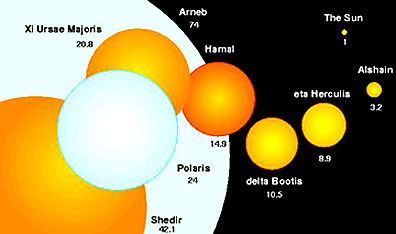
Most stars bigger than the Sun are not as huge as Mu Cephi or Epsilon Aurigae. The majority are no larger than about 100x the diameter of the Sun. This diagram illustrates the relative size of some common stars (setting the Sun’s diameter as 1), which establishes our star as rather ordinary in the size scheme within the Milky Way:
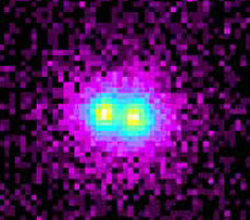
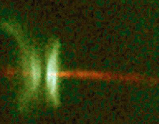
More than half of the stars in a galaxy are also tied locally to a second star as a companion (binary), such that each of the pair or group orbits around a common center in space determined by their mass-dependent mutual gravitational attraction. This arrangement is exemplified by the image made by the HST Faint Object Camera (FOC) of the Mira star (Omicron Ceti) in the Constellation Cetus.
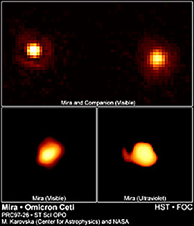
This star is a Red Giant (see below) which appears to be periodically brightening (it is credited as the first known variable star, having been discovered in 1546 A.D.). The HST has resolved it into a binary in which the star on the left has a White Dwarf (see below) at its core and now receives mass from the Red Giant that accumulates until the hydrogen burns (see first illustration at the top of page 20-6). An ultraviolet (UV) image made by HST’s FOC actually shows mass being drawn off the Red Giant.
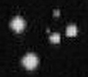
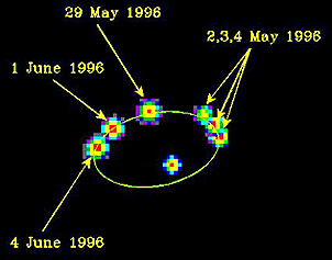
Some stars are grouped into more than one companion; ternary groupings (three stars orbiting about a common center of gravity) are fairly common. Here is an image of four stars orbiting as a unit about a gravity center in the galaxy M73.
Binary star systems are recognized by three means: 1) visual, through a telescope (as in the above two images); 2) by periodic drops in brightness caused by passage of one star across another (eclipse; an uncommon observation condition); and 3) by measuring spectral characteristics in which both a Doppler shift towards the red and the blue occur as one star moves away and the other towards Earth (and the reverse) along pathways of their mutual orbits.
To demonstrate the second means, examine this diagram which shows the brightness levels (and magnitude variations) for the binary star Algol:
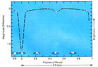
The larger star (in blue) is mutually orbiting a smaller star (red) which has a notably smaller output in its own luminosity. When the latter star passes in front of the larger star, there is a notable drop in the combined luminosities, as the partial eclipse cuts out some light from the larger star. Then, when the red star passes behind the blue star, there is a small drop in luminosity since the smaller, now occulted star does not send any of its light to the observing telescope.
Spectral line shifts are used to study the motions of binary stars. We will treat stellar spectroscopy in detail on page 20-7 As a preview, the spectral method can be illustrated by looking at a pair of spectral strips for two similar stars that are mutually orbiting:
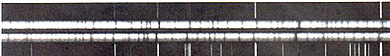
Bright lines for hydrogen appear in the top and bottom (dark background) strips. This fixes a reference location for excited hydrogen in the rest state. The two center spectral strips include the same hydrogen lines, the first strip acquired from one and the second the other star. Note that the lines in one have moved to the left and the other to the right of the reference lines position. The spectrum on the bottom center has been blueshifted (see page 20-9) towards shorter wavelengths; the spectrum at the top center has been redshifted towards longer wavelengths. This is explained thusly: The bottom star is in motion towards the observing system on Earth whereas the top star is moving away from the telescope. This would occur when the two stars are aligned sideways to the line of sight and are moving in opposite directions around a common center of gravity.
For some visual binaries, movements over time can be observed and plotted, such as illustrated here for the star Mizar (in the Ursa Major constellation), which is resolvable into Mizar A and Mizar B.
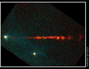
The Chandra X-ray Observatory has imaged a close binary pair in the M15 Galaxy. Prior to obtaining this image, the object was thought to be a single star, but at x-ray wavelengths, it is now resolved into a faint blue star and a nearby companion believed to be a neutron star giving off high energy radiation. Thus:
Turning now to stellar evolution, to preview what will be examined in some detail (shown in chart form later on this page), the pattern of a star’s history follows a pathway that, depending on its total mass, eventually splits into one of two branches (/> or \>), as it leaves what is known as the Main Sequence. This is: Development of a large cloud of denser gas made up of predominantly molecular hydrogen (H:sub:2) + dust –> Protostar –> T-Tauri Phase –> Main Sequence /> (if mass less than 8 solar masses)–> Red Giant –> Planetary Nebula –> White Dwarf; OR \> (if mass greater than 8 solar masses) –> Supernova –> Neutron Star and/or Black Hole (depending on mass [size]).
Both star classification and evolution can be summarized in a graphlike chart that consists of a plot of luminosity (vertical axis) versus star surface temperature which is expressed also by (correlated with) the star’s visual color (note also the Spectral Type designations at the top). This is known as the Hertzsprung-Russell (H-R) Diagram. Mass densities are shown as numbers on the the central line that defines the Main Sequence (M.S.) of stars. Most known stars lie along this line; they describe a stage in which a star reaches some fixed size and mass and commences burning of most of its hydrogen before changing to some other star type off the sequence. Star types, which are defined on the basis of stellar surface temperatures page 20-7), are shown by the letters (O, B,…etc.) assigned to each group and evolutionary pathways for some are indicated. This particular plot also shows along the right ordinate the total time that Main Sequence stars of different masses spend on that sequence before evolving along the several principal pathways (see below); as far as we now know, stars do not completely vanish, but survive as dwarfs or Black Holes ( but the latter in principle can disappear by evaporation as Hawking radiation).

From J. Silk, The Big Bang, 2nd Ed., © 1989. Reproduced by permission of W.H. Freeman Co., New York
In the version below of the H-R diagram, the various major star types or states for stars that are not on the Main Sequence are shown (the spread of those types as a function of temperature-luminosity variations is plotted). Among the off-M.S. evolved star groups are four types of Giants (Sub; Red; Bright; Super), T Tauri; and the two major types of cepheids. These are discussed again on this page or elsewhere in this Section. Not shown is the recent designation of LT for Brown Dwarfs. Note that the letters at the bottom include some like B0 and B5 or K0-K5; this denotes subdivision of each class into temperature subclasses (0 being hottest and 5 coolest in a class). Temperature ranges (in °K) are: O class = greater than 30000; B = 11000 - 30000; A = 7500 - 11000; F = 6000 - 7500; G = 5000 - 6000; K = 3500 - 5000; M = less than 2500. Colorwise, the first three are all “blue-white” stars, F is bluish to white; G is white to yellow; K is yellow orange; and M is red.
This next diagram is another H-R variant in which some well-known stars with specific names (visible to the naked eye or through a telescope) have been plotted. The Red Dwarfs and Blue Giants are specified in this version. On the right is the size of a star (in terms of radius) relative to the Sun taken as 1.:

This diagram shows the sequence star stages from a nebular mass into a protostar, then to the M.S., and on to a final dwarf state for a sun-size G star.

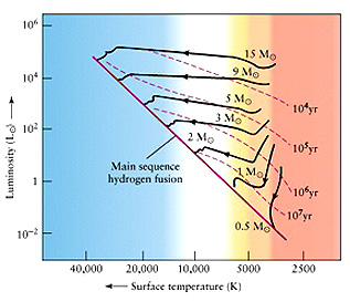
The pathways of protostars to the Main Sequence, as shown on this modified H-R diagram, depend on their mass (in multiples of a solar mass) at the stage when they commence proceeding to the M.S and initiate hydrogen fusion. The times involved in this transition will vary systematically with mass; thus, a 15 solar mass protostar takes only about 10000 years to reach the M.S. whereas a 2 solar mass star may require up to 10,000,000 years for the process to begin fusion:
This next diagram shows the evolutionary history of three stars at the upper, central, and lower ends of the Main Sequence after they leave the M.S.:
|Pathways of change after 3 Main Sequence stars (of greater, equal to, and less than a solar mass) depart from their dominantly hydrogen-burning phase. |
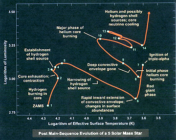
These pathways are somewhat generalized. When the details are plotted, the path of a star of 5 solar mass size from the M.S. to a Red Giant can be more complex, as shown in this multi-step example:
The largest number of individual stars in galaxies fall between just under 1 solar mass to about 10 solar masses. As these burn their hydrogen fuel into helium, as they begin to burn the helium they brighten, cast off some of the outer hydrogen, and become luminous (for stars under a solar mass of 2.3, there is a short-lived large increase in luminosity known as the helium flash phase). Then, as the helium burns to carbon (which organizes into a core of degenerate C and some O; see page 20-7), such stars follow what is known as the asymptotic giant branch (AGB) pathway which begins with a second Red Giant state. That is shown in this diagram (as well as the three previous diagrams):
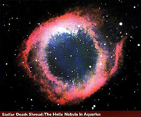
This shedding enroute to the planetary nebula phase (further described below) can appear in a spectacular manner, as shown by this HST image of the Helix Nebula, in which the red ring is excited hydrogen:
A star’s precise position along the Main Sequence depends on the total mass of H fuel that collects during the formative phase into the gas ball. Some stars (e.g., Type M) have masses as low as 1/20th of the Sun (1 solar mass is the standard of reference as is the luminosity of the Sun, also set at 1), whereas others fall within a range of greater masses that may exceed 50 solar masses (Type O). The high mass stars on the Main Sequence are brighter and bluer whereas those at the lower end of the M.S. tend to be yellow to orange. The initial quantity of mass in a star is the prime determinant of its life expectancy, which also depends on its evolutionary history and final fate. As a general rule, small stars may take more than 50 billion years to burn out completely, stars in the size range of the Sun live on the order of 5 to 15 billion years, and much bigger stars carry their cycle to completion in a billion or less years. Stars whose masses are similar to the Sun’s actually will burn about 90% of their hydrogen during their stay on the Main Sequence. Stars with greater than 50 solar masses may complete their M.S. burning in just 20-30 million years.
The lifetime spent on the Main Sequence is approximately proportional to the inverse cube of the star’s mass (this is true for most stars, especially massive ones; stars less than a solar mass have lifetimes closer to the inverse 4th power). The relation between size (mass) and age is shown in this next diagram:
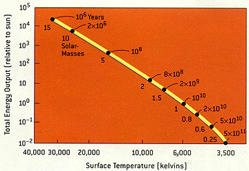
From B.C. Chaboyer, p. 53, Scientific American, May 2001
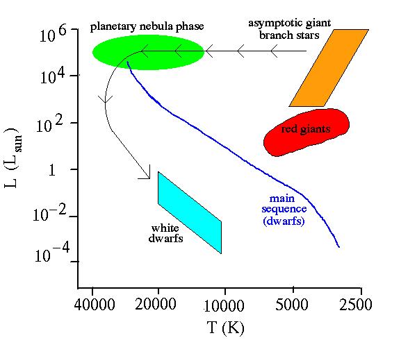
The fate of stars (at the end of their history) of all sizes (and different masses) can be conveniently summarized in this Evolution diagram:
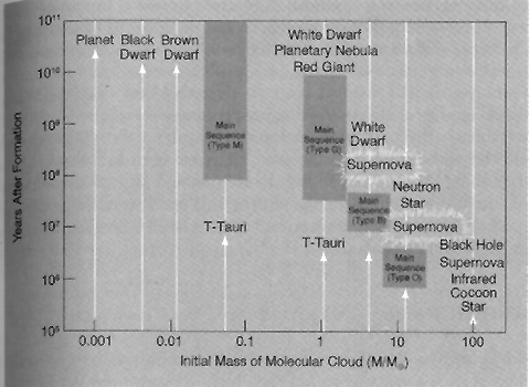
From J. Silk, The Big Bang, 2nd Ed., © 1989. Reproduced by permission of W.H. Freeman Co., New York
A variation of this diagram (which unfortunately does not produce well when reprocessed after being taken off the Internet) is included here because of its pictorial wealth of information:
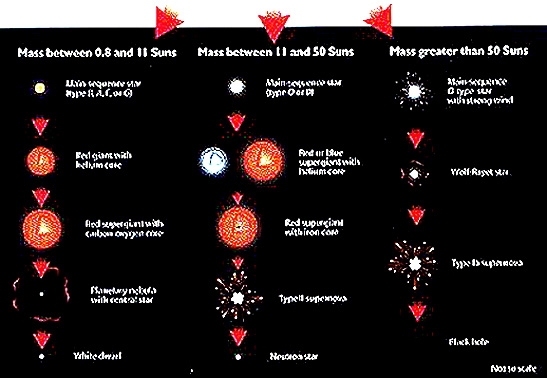
Of special interest are the end products of each evolutionary path. After burnout or explosion, small stars end up as White Dwarfs; intermediate stars as Neutron Stars; and the largest stars as Black Holes.
Now to a more detailed discussion of the history of stars as expressed in the above diagrams.
Stars develop within galaxies in nebulae (also called Giant Molecular Clouds [GMC] composed mostly of H2) by progressive sub-fragmentation, aggregation and contraction of gas and dust into centers of higher density. These nebulae represent localized concentration of gases brought about by several processes such as the driving force of shock waves from supernova explosions and intergalactic magnetic fields. The clouds turn very slowly but this helps to develop “seed” locations - internal denser regions that bring the gases toward them because of greater gravitational attraction. The H-He atoms in these denser local regions assemble into gas balls and dust clouds by collisions and gravitational forces at initially low temperatures (100’s of ºK) in a turbulent process of condensation, generating heat (in large part dissipated as thermal radiation). Thus, molecular hydrogen clouds are the regions of gas where most new stars are born.
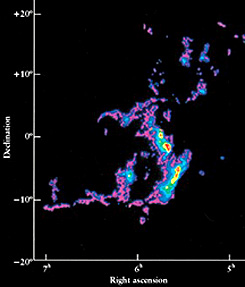
One way to study GMCs is to plot the distribution of excited carbon monoxide (CO) dispersed within the molecular hydrogen. In this state CO produces two prominent emission lines at 1.3 and 2.6 mm in the near radio wave segment of the EM spectrum. (H:sub:2 does not emit strong signals in the radio region.) Here is the CO pattern that occurs in the Orion Nebula (a GMC which also contains strong HII (ionized H) regions (see below)
Outside the clouds, H and He also are dispersed, at much lower densities, as the principal elements distributed in interstellar space; the density of free H (mostly neutral) in that space is estimated to be between 3 and 8 atoms per cubic meter. This atomic hydrogen when excited but not ionized is detectable by its signature at a 21 cm wavelength as determined through radio telescopy, representing photon radiation given off when excited hydrogen reverts to its lowest energy state. But, in spiral galaxies most atomic hydrogen gas has been rearranged in long streamers between arms of existing stars, as seen in this 21-cm radio telescope image of the Milky Way.
When GMCs heat up to temperatures above about 5000° K, the hydrogen can be ionized (see Page 20-7 for a discussion of the different ionized states of hydrogen and their characteristic spectral lines). This gives rise to strongly emitting clouds that are referred to as H:sub:`II` Regions (Atomic hydrogen is denoted by HI; alternate forms of this symbol are H II or HII). One prominent line used to image and study HII regions is Hα, whose line lies at 0.656 µm - the N3 –N2 transition in Balmer series. These clouds are photogenic and deserve several examples here. First, an emission nebula as imaged by a telescope used in the 2Mass project (inventory of stellar objects in the Visible-Near IR):

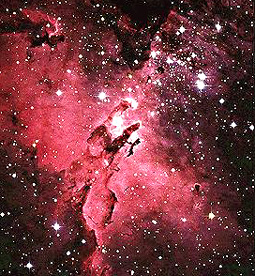
We follow this with an image of part of M16 (Eagle Nebula) that has heated to the HII temperature range, with colors chosen to indicate that HII clouds also are bright in the Near-IR:
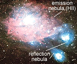
And lastly, an image which contains an emission cloud (pink) and two smaller reflection clouds (molecular hydrogen) (blue):
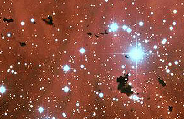
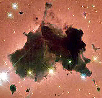
Before organizing into an galaxy or after a galaxy has formed, the initial nebulae will have irregular shapes. Some nebulae appear dominated by dark dust, mixed with hydrogen. These may have elongated shapes, some of which are described as “pillars”. Part of the Eagle nebula contains such dark dust concentrations, as seen here:

A close view of one of these pillars (said by many as the most fascinating image yet obtained by the HST) is shown on page 20-11. Another type of dark dust-rich clot, with sharp boundaries, of star-forming material is called a “Bok Globule” (see several examples on Page 20-4), which commonly produces a large number of massive O-type stars, the brightest on the Main Sequence, which have short life times. Here is a typical grouping of dark patches that belong to the Bok Globule category:
A pair of Bok Globules in IC 2944 appear to be merging in this HST close-up:
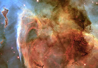
Now look at part of the Keyhole nebula, some 8000 light years from our own galaxy. Its size is about 200 l.y. in diameter. It is classed as a dark nebula, but in this rendition computer processing brings out its rich colors. (Note: the term nebula, derived from the Latin for “cloud”, has multiple meanings. In the early 20th century, the word was applied to bright objects in the sky that Hubble and others showed to be galaxies; now, the term is restricted to any collection of hydrogen gas and dust that may occur outside of a galaxy, as intragalactic material, or as remnants of exploding stars.) A good review of the types of nebulae is found at The Web Nebula.
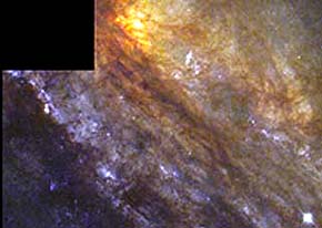
A typical gas and dust cloud (as shown below, a subsection within a developing spiral nebula, NGC253) consists of a number of bright, bluish new stars midst swirls of hot hydrogen-rich gas, and some older stars.
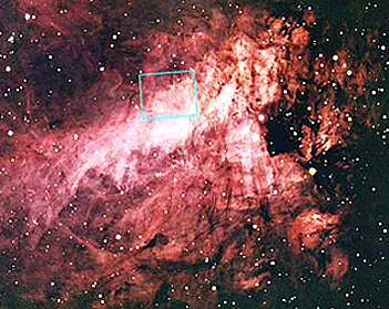
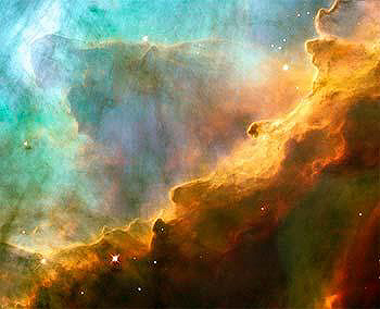
This next pair of images confirms once more the value of HST in providing details about astronomical features. The first image of the Swan Nebula, M18, some 5000 light years from Earth, was taken from the Anglo-Australian ground telescope. The box indicates the area imaged by the HST Wide Field Camera, showing an almost 3-D like view of the clouds in this small part of the nebula. Red colors indicated excited sulphur; green in this rendition is hydrogen gas (in other renditions using different color filters H is often shown in red), and blue associates with oxygen.
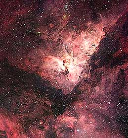
One of the largest nebulae is the Carinae nebula, seen only from Earth’s southern hemisphere. It is a bright nebula (and contains the supernova Eta Carina star) that lies just beyond the above Keystone nebula.
As a large number of stars develop from a nebula, and become luminous as hydrogen-burning ensues, processes including radiation pressure from starlight will allow the stars to be seen through the diminishing dust and gas. The nebula may continue to produce more new stars if it draws more hydrogen from beyond its boundaries, but generally nebulae tend to use up available H2 and may deactivate. Stars may then form elsewhere as new clouds develop and reach conditions favoring stellar generation.
Individual stars develop along fairly well known blueprints. A central clot of mainly gas organizes and is surrounded by an envelope usually enriched in dust. As the protostar heats up, some of its material is ejected by magnetic forces as jets, such as in these two examples:
The expulsion of these high speed gases and charged particles can cause parts of the surrounding nebular masses to be excited and glow in luminescent patches. This phenomenon is known as Herbig-Haro (HH) Objects. Here is one example:
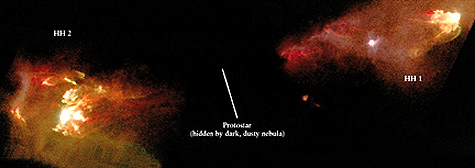
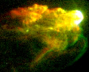
The emergence of these objects at two opposing sides (bipolar) of the protostar is typical. The next HST view shows this HH effect in a glowing “cloud” which is located near the end of a jet (bright hemisphere, to the right) passing through it.
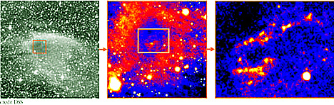
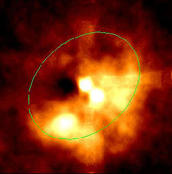
In the nascent star phase, the dust and gases form a very large volume of organizing material called a “globule” (at least some of these are Bok Globules; see above). A globule in the inner Milky Way, designated DC303.8-14.2, shown below was first detected by ESA’s IRAS satellite. In this trio of images, the left image of the globule, obtained during the Digital Sky Survey observations, shows the extent of the nebular mass seen in visible red light. The center image made by Kimmo Lehntinen’s team using VLT ANTU telescope at ESO’s Observatory in Chile, is the inset of the left image shown here in color from several infrared band images on this telescope, It shows a distinct ring of gases and dust that emits strongly in the infrared. The right image (of the inset of the center image) indicates several jets of the Herbig-Haro type involved in the early stages of formation of the eventual star.
From the above discussion we conclude that the dominant behavior during the pre-Main Sequence history of a protostar is marked by light gases continuing to inflow and build up the star’s mass and size. Much of the dust remains as a thick disk outside the star, such as this example:

As will be further explained on page 20-11, disks like this are the potential conditions that lead to planet formation. Meanwhile, the star approaches pressure-temperature levels capable of initiating hydrogen fusion, as described in the next paragraph.
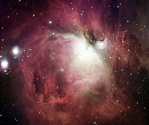
As more matter accrues within a growing nebula, its internal gravity continues to increase and draw in still more gases. Gravitationally-driven collapse into forming stars induces compression and further heat rise. The protostar phase is reached as temperatures rise to 2000 - 3000° K. At ~10,000° K, the H begins to ionize (electrons stripped away) and, in the process, loses some heat energy by radiation which tends to slow or counter the compression. Over time, the cloud eventually reaches a density that requires it to then undergo local clumping of gases into clots that grow into still denser concentrations to become stars (these smaller clots can exist for much of the galaxy’s life but are the sites of further star formation). Here is a Hubble Space Telescope (abbreviated as HST and described on page 20-3) view of the Orion nebula, which appears to be in an early stage of organization into stars (hence, a younger nebula).
Here is a gas cloud in the Orion nebula as seen by HST’s Wide Camera; but on the right is the same area imaged in the IR in which a bright small star “shines through” as a protostar.

Seen close-up is the central part of Orion, in which the reds are related to the excitation of hydrogen gas (using a red filter on the HST image).
In July, 2003 a report was released stating that the Orion nebula contains the hottest stars yet discovered in the Universe. Temperatures were obtained using Chandra X-ray data. The 3 hottest were supermassive stars shown in the right panel below:

The hottest of these reached a surface temperature of 60 million degrees Centigrade (108,000,000° F), more than double the value of the previous record holder.
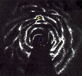
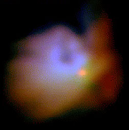
As the early stages of star formation proceeds, the cloud tends to gather around the star in a more isolated manner, removed from neighboring gas and dust nebula. It may then enter the T Tauri phase at which the growing star starts to generate strong stellar winds. The cloud disk still can exceed 150 A.U. in dimension. This telescope image shows the glowing cloud (rendered here in blue, but actually of a different color) around the incipient, still poorly organized central star (a binary pair).

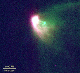
Here are two more T Tauri stars, the one on the left showing the nebular shield that masks the bright growing star and the one on the right showing another T Tauri star as seen in the infrared:
The star now rapidly contracts as it passes through the Hayashi phase. This relies on the proton-proton nuclear reaction which releases radiation energy that causes a notable increase in luminosity. However, hydrostatic equilibrium (see below) is not yet reached as the growing star continues to experience disruptive convection.
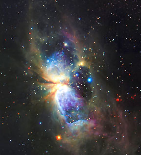
This next view shows a star after most of its accretionary disk material has been incorporated into its mass, as it nears the stage where it will be on the Main Sequence.
For stars of masses near that of the Sun, it takes about 10 million years to work through the protostar phase and another 20 million years to join the Main Sequence. More massive stars reach the Main Sequence more rapidly. Below is a view taken through the Japanese Suburu Telescope of S106, with mass twenty times that of the Sun, which began to burn only about 100,000 years ago. This star, 2000 l.y. from Earth, still is showing dust and gas flowing into the central body.
An early stage of another massive star, AFGL2591, 10 times the size of the Sun, has been viewed in infrared light by the newly operational Gemini North Telescope on Mauna Kea, Hawaii. Some 3000 l.y away in the Milky Way (located against the backdrop of the Constellation Cygnus), the central region of the forming star is still disorganized. Infalling material continues its growth but also sets off a return outflow of gas and dust.
|The Giant star, AFGL2591, seen through the Gemini North telescope, and imaged in the infrared.<font |
After a star has moved onto the Main Sequence, the history of its life cycle there will be a continuous (somewhat oscillating) “contest” between contractive heating during stages of gravitational collapse and expansive cooling by thermal radiation outbursts whenever rising temperatures increase hydrogen ionization. Generally, an evolving star tends to seek out a balance [hydrostatic equilibrium] between inward gravitational forces and outward radiation pressure developed from the burning of the star’s nuclear fuel. This is illustrated in this simplistic diagram:

In its early life, the contraction phase ultimately dominates, so that a star’s deep interior temperature eventually will be raised above 107 K (varies with star size), at which stage a fundamental nuclear reaction within the hydrogen gas commences. This involves thermonuclear fusion: p + p => H2 + e+ + neutrinos (H:sup:2 or deuterium is a single proton and a neutron and e+ is a positron [emitted]). That change of state results in thermal energy release which contributes to continual rises in temperature. Deep within the star, an alternate but dominant fusion process involves melding of 4 single protons into a single helium nucleus consisting of two protons and two neutrons. As temperatures increase further, some protons, neutrons, deuterium (and minute amounts of tritium [H:sup:3]) combine (in a three step process) into helium (He:sup:4 nuclei [2p, 2n]) which migrate into the star’s interior towards its core. In these reactions, some of the mass is converted to energy (E = mc2) which radiates outward as the source of the star’s luminosity and which produces the outward pressure that counteracts inward forces owing to gravitational contraction. Luminosity varies as the fourth power of a star’s mass (thus a star with twice the mass of the Sun shines 16 times brighter).
Helium remains stable until temperatures approach 100 million° K, at which state it reacts with more protons and neutrons to transmute into other elements of higher mass numbers (see below). More massive Main Sequence stars can generate Carbon; some of this element may be in the star initially if it is formed from previous gases and particles that contain carbon produced in earlier star generations. This carbon-enriched star, as its temperature rises and interior pressure increases, can go through another fuel-burning process known as the CNO. Through a series of steps as reactions of Carbon with Hydrogen protons take place, first C12 is converted to isotopes of Nitrogen or O15 but reaction with He4 will lead to C12 again plus energy released as positrons and neutrinos.
When the H => He process reaches a steady state, gravitational contraction no longer dominates (attains a balance called hydrostatic equilibrium)), the star’s total radiant (EM) energy output per second (defined as its luminosity; also referred to as brightness) becomes constant, and the star reaches a stable state on the Main Sequence (M.S.), populated by stars that are primarily in the hydrogen-burning stages. This equilibrium - in which inward directed gravity forces are more or less countered by outward radiation pressure - is maintained during most of the star’s life on the Main Sequence. These stars spend up to 90% of their total lives on the Main Sequence.
Because this page is very long and has so many illustrations that downloading is lengthy, the second half (remainder) of the page on Stars is continued on page 20-5a, accessed by the Next button at the bottom here and at the top of this page.