The Klamaths from Space
The Klamath Mountains of Oregon are described and visualized through ground photos. The conventional geologic map (rock units are mapped but the context is not that of terrane units) is shown and the map that characterizes the assemblage of stratigraphic units as distinct terranes is presented. DEM data are used to make shaded relief portrayals of all of Oregon and of the Klamaths within. The strategy guiding the study is stated in terms of the principal parameters to be measured, both by standard geomorphic methods and through use of space imagery.
The Klamaths from Space
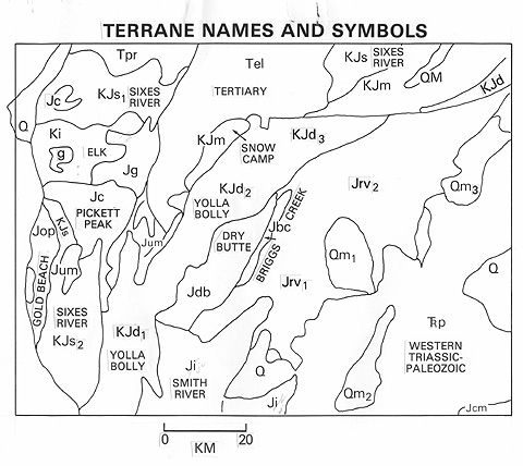
As a visual aid to realizing that there are distinctly different terranes, we reproduce here a simple map (unlabelled) that assigns a different color to each terrane. Match with the map above. The easternmost terrane shown is Jrv, which stands for Rogue Valley (inadvertently left out of the sketch map). Yellow denotes Quaternary deposits - both river and lowlands fill.
positioned on a computer-generated map to better indicate to the eye their distribution.|
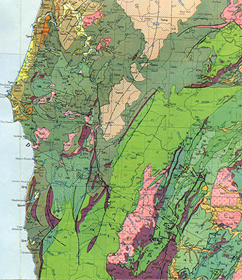
you may be able to see a close correspondence between some units and their enclosing terranes, a broader correspondence for others, a number of individual units that are scattered about within the terranes, and some units that seem to cross over or overlap terrain boundaries. Because there are so many units [generally, at the formation level], I don’t show the map’s legend. Also, in the legend sequence are units that aren’t present in the Klamaths. Two examples of exceptions are the deep purple unit (Jui), which is actually outliers of ultramafic (ophiolitic) lavas, once part of oceanic crust, which appear similar in the field but originated locally within their terranes, and the pinkish-red unit, which consists of intrusive rocks that invaded several terranes, already in place. One expects this general agreement between terranes and their constituent stratigraphic units (i.e., internal consistency), along with the exclusivity of some units to single terranes, inasmuch as terranes typically develop from rocks formed in different source areas at different times.
` <>`__17-17: Although it will require considerable scrolling up and down on this page, go ahead and try to match the different color units in the geologic map with the terrane units in the map above. `ANSWER <Sect17_answers.html#17-17>`__
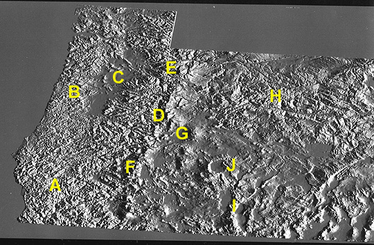
Features of interest in this shaded map are: A = Klamath Mountains.; B = Coast Ranges; C = Willamette Valley (Portland at the north end); D = High Cascades; E = Mount Hood; F = Crater Lake; G = Paulina Mountains (Newberry Crater); H = Blue Mountains.; I = Abert Rim; J = Summer Lake area (the circular area is somewhat an artifact of the illumination)
You can get a feel for the appearance from the ground of several of the Klamath terranes through these photographs taken during the writer’s time in the field:
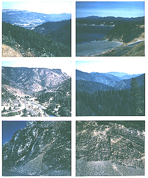
The upper left scene shows terrain around Canyonville, with Yolla Bolly terrane in the foreground and Sixes River terrane in the distance. Next to it is a view from the coast of the Elk terrane. In left center is a segment of a canyon dissected by the Rogue River, in which sedimentary units of the Rogue Valley terrane (Jrv) are exposed. To its right is landscape typical of the higher elevations in the Klamath Mountains. The lower left scene is an exposure of serpentinite (the metamorphosed ophiolitic basalts associated with oceanic crust). The lower right shows alternating layers of siliceous (cherty) shales that constitute island arc sediments. Here they are part of the Yolla Bolly terrane.
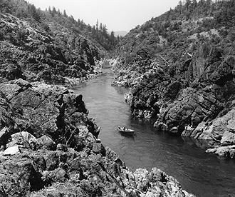
The wildest part of the Klamaths is the Rogue River which cuts deep canyons into the rocks. This is one of America’s premium whitewater rafting streams. This photo captures it ruggedness:
We proffer a preview of the topographic expression of the Klamath Mountains, which will be presented in Landsat format shortly, by this enlargement of the area made from the same DEM data. Notice Crater Lake (nearly circular on top of a mountain) in the upper right part.
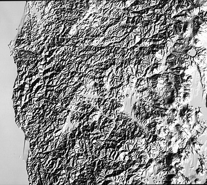
The terrane map is reproduced here again to aid you in matching units to their DEM expression. Keep in mind that the DEM version covers a notably wider area.

In this visual version, we have trouble seeing any significant variations in terrain that call attention to noticeable terrane differences. Of course, we can vary the illumination directions to emphasize contrasted ridge and valley orientations, We did vary the illumination directions on this data set, giving several distinct expressions but, again, obvious patterns that correlate with the various terranes as mapped did not stand forth. However, when one learns where to look, after familiarization with terrane locations, strong hints of certain differences for several of the terranes are discernible. These differences can also be disclosed by appropriate analysis of topographic data in map-sheet or DEM formats and, in fact, this approach proved superior to visual differentiation.
The reason we would postulate for expected differences is that each terrane consists of a group of rock types that will likely differ from other nearby terranes. Fault discontinuities also bound each one, at least partly. A terrane will respond to regional erosive action according to its mix of lithologies. Thus, any one terrane may develop landform characteristics that differ from its neighbors and can appear visually as separable. We should be cautious about expecting the differences to remain neatly within terrane boundaries, because, as the landscape develops within any one terrane, the equilibrium forms tend to exert some influence on terrains outside the boundary. Nevertheless, the hope in testing the hypothesis of distinctive terrane-controlled topographic expression is that real differences do occur.
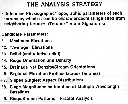
This effort is predicated on making a series of quantitative measurements that can be tested numerically and statistically to ascertain valid differences in the topographic character of each terrane. In general, it is quite difficult to extract any of these measures with confidence from Landsat imagery. However, one overlapping SPOT image pair was available, so that a stereo image is achieved, allowing limited recovery of measurable variables. So, in the exposition that follows, Landsat’s prime role is to help to confirm the terrane-terrain association by visual recognition.