Multisensors
Contents
Here we delve into the advantages of multisensors. This leads to a discussion of merging an image produced by one sensor with that of another. Both may cover the same wavelength range but differ in, say, resolution or pixel size. Or they may be quite different types of sensors, e.g., radar and visible band scanners.
Multisensors
A word that naturally springs from the “multi” concepts is merge. Data acquired by different platforms, with different sensors, at different resolutions, and during different times will tend to be incompatible in some respects. Most common is geometric: the pixel representing radiometric data in some spectral interval from some area on the ground or in the atmosphere will probably not be the equivalent size for the different sensors that monitor the target, be it the Earth’s or a planetary surface, or the properties of the air above. In order to combine data sets from different sources, some adjustments or shifts in both geometric/geographic and radiometric values will be required. Two pixels may partially overlap; they may vary in shape. Their radiometric character may require modifications (e.g., correcting for atmospheric effects or for bidirectional reflectance). Thus, to successfully merge, both geometric and radiometric corrections must be applied. Some form of resampling (see page 1-12) is usually necessary. Distortions must be reduced or removed. Rectification to some planimetric standard (for example a suitable map projection) has to be incorporated. And fitting or stretching one image to properly overlay another is often vital, requiring ground control points or tie points. These general processing steps, while vital, will remain beyond the ken of this Tutorial but the interested user should consult any of the textbooks listed in the Overview, as, for example, the just published 5th edition of Lillesand and Kieffer’s Remote Sensing and Image Interpretation. On this page we must be content with looking at some examples.
The first continues the last themes of crop fields and radar. Below is a SIR-C image of fields in the Red River basin of Manitoba. Two of the bands in the color composite are from the L- and C-band radar systems operated by JPL. The third is the X-band instrument developed by a German-Italian space consortium. All were mounted on the boom that extended from the Shuttle. Since the images were taken simultaneously, the time factor is eliminated. But the two instruments were not completely compatible in spatial sampling, so the pixels required appropriate algorithms to permit merging, and in some instances difference in look angles and polarization.
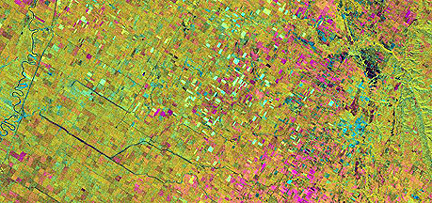
The fields were producing mostly corn, wheat, barley, sugar beets, and canola. Magenta designates bare soil; bright fields are dominantly corn; other standing biomass is in cyan.
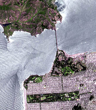
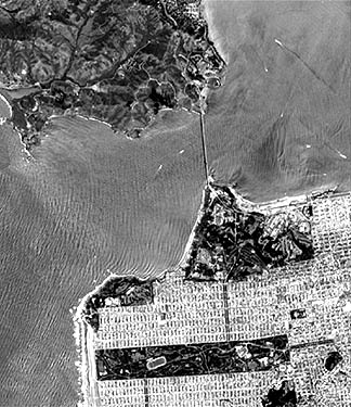
SPOT provides excellent examples of fairly simple merging: the 20 m HRV multispectral data with the 10 m HRV Pan(chromatic) sensor. The first two paired scenes show part of San Francisco, including the Golden Gate Park, the Presidio, the Golden Gate bridge, and Sausilito in Marin County. The image on the left is a 20 m quasi-natural color view; on the right is the black and white 10 meter resolution image of the same area. Both scenes were acquired at the same time.
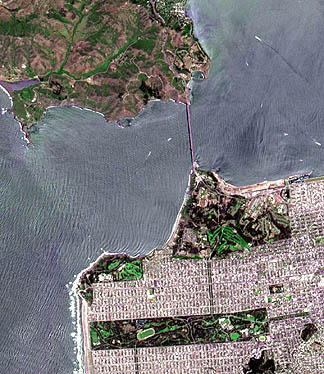
Now, in this next scene the two are merged:
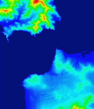
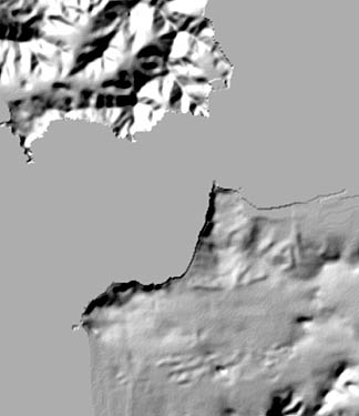
In previous Sections, we have shown several examples of combining space imagery with DEM elevation data to produce perspective views. We can do this with the above scene. First, the DEM data are displayed in a color coded general map, with high elevations in red and lowest in medium blue (ocean dark blue). They are then input to a shaded relief map, on the right:
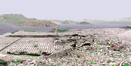
After registration of the image pixels with DEM data points, and the appropriate procedural algorithm, the scene is converted to the following perspective view:
Several more merge scenes round out the picture. The next fuses a Landsat TM color composite at 30 m resolution with and IRS (Indian remote sensing program) 5 m panchromatic image of an unnamed town, with impressive results:
|Merging of a 30 m Landsat TM color composite with a 5 m IRS panchromatic image of the same area. |
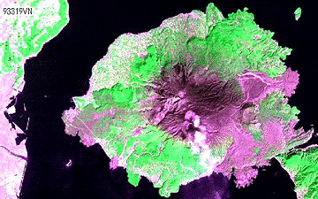
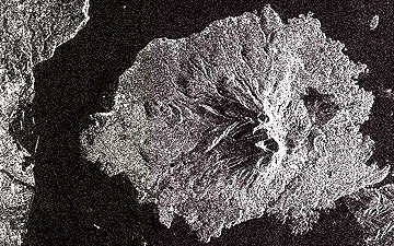
The next pair of images were taken simultaneously from the same JERS platform but the instruments are quite different. The top image, depicting Mt. Sakurajima (volcano) in Japan, is made from OPS (Optical Sensor), a multispectral instrument that has an 18 x 24 m resolution and covers a swath width of 75 km. The bottom is an L-band SAR image, with 18 m resolution and the same swath width. The two images are shown here as separates but can be easily merged.
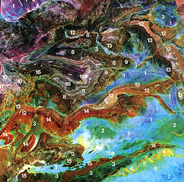
Thermal imagery also benefits from merging with other kinds of images. This next image, made by Rupert Hadyn, contains color information relating to temperature variation in the mountains of Morocco. The input data are Day-VIS, Day-IR, and Night-IR readings from HCMM, shown in a color composite that uses the IHS (Intensity-Hue-Saturation) color system. The resulting color image has been registered to a Landsat MSS Band 5 scene of the same area, so that its black and white appearance gives a sense of topographic expression superimposed by colors, such that reds are associated with the warmest night temperatures and blues are the brightest areas in the Day-Vis scene.
Primary Author: Nicholas M. Short, Sr. email: nmshort@nationi.net