Accuracy Assessment
Contents
Several kinds of errors - mainly those of “commission” or “omission” are discussed as a basis for setting up an accuracy assessment program. Accuracy itself is defined and the point is made that much depends on just how any class, feature, or material being classified is meaningfully set forth with proper descriptors. Two factors are important in achieving suitable (hopefully, high) accuracy: spatial resolution (which influences the mixed pixel effect) and number of spectral bands involved in the classification. A case study in the Elkton, Maryland area is treated in some detail to demonstrate just what the accuracy of its classification in Landsat data sets really means.
Accuracy Assessment
Of course, in the real world many classes or features are not homogeneous, that is made of one material and formed in one definitive shape. Consider the class “field”. During a growing season, the field is a mix of soil, crop(s), and some degree of moisture (ephemeral). There are many types of soils, which vary in color, composition, and texture, and crops also range in variety and density (absence = fallow field). Another class is “urban,” which can include a diversity of buildings made of different materials, in various sizes and shapes; roads formed of concrete or asphalt; trees and grass, and other variables. We can often further subdivide the classes into more specific categories, such as “saturated field of corn” or “shopping center”, provided they correspond closely to unique or distinctive spectral signatures, as determined in establishing prototypical training sites. This internal mix of several substances or features that are intrinsic to a class, does not have the same meaning as the resolution-dependent straddle-mix of several classes described above.
` <>`__13-6: Consider this class: “factory complex”. In this case, it occupies a non-residential part of suburbia. Break it down into the likely components (internal mix) that are present, even though it is implied by its name to be a single unit. `ANSWER <Sect13_answers.html#13-6>`__
Some elements of the ideas from above became clear to the author during his first experience in the late summer of 1974, while going into the field to check on an unsupervised classification made by the LARSYS (Purdue University) processing system and to designate new training sites for a subsequent supervised one. The classified area centered on glacial Willow Lake on the southwestern flank of the Wind River Mountains of west-central Wyoming. Prior to arriving onsite, we prepared a series of computer-generated printouts (long since misplaced), in which an alphanumeric symbol represented each spectral class (separable statistically but not identified). Different clusters of the same symbols suggested that discrete land use/cover classes were present. In the processing, we allowed the total number of classes to vary. Printouts with seven to ten such classes looked most realistic. But there was no a priori way to decide which was most accurate. In touring the area, we had to revise or modify our preconceived notions about classes. We had not considered the importance of grasses and of sagebrush, nor anticipated clumps of trees below the 79 m (259 ft) resolution of the Landsat Multispectral Scanner. After a tour through the site, the author gazed over the scene from a slope top and tried to fit the patterns in the different maps into the distribution of features on the ground. The result was convincing: the eight-class map was mildly superior to the others. Without this bit of ground truth, we would not have felt any confidence in interpreting the map and deriving any measure of its accuracy. Instead, what happened was a “proofing” of reliability for a mapped area of more than 25 square kilometers (about 10 square miles) through a field check of a fraction of that area.
We may define accuracy, in a working sense, as the degree (often as a percentage) of correspondence between observation and reality. We usually judge accuracy against existing maps, large scale aerial photos, or field checks. We can pose two fundamental questions about accuracy: Is each category in a classification really present at the points specified on a map? Are the boundaries separating categories valid as located? Various types of errors diminish the accuracy of feature identification and category distribution. We make most of the errors either in measuring or in sampling. Three error types dominate:
Data Acquisition Errors: These include sensor performance, stability of the platform, and conditions of viewing. We can reduce them or compensate for them by making systematic corrections (e.g., by calibrating detector response with on-board light sources generating known radiances). We can make corrections, often modified by ancillary data such as known atmospheric conditions, during the initial processing of the raw data.
Data Processing Errors: An example is misregistration of equivalent pixels in the different bands of the Landsat Thematic Mapper. The goal in geometric correction is to hold the mismatch to a displacement of no more than one pixel. Under ideal conditions, and with as many as 25 ground control points (GCP) spread around a scene, we can realize this goal. Misregistrations of several pixels significantly compromise accuracy.
Scene-dependent Errors: As alluded to in the previous page, one such error relates to how we define and establish the class, which, in turn, is sensitive to the resolution of the observing system and the reference map or photo.
Three examples of these errors come from a common geologic situation (also treated to some extent on page 2-5), in which we process the sensor data primarily to recognize rock types at the surface. In this process there are pitfalls:
First, geologists in the field map bedrock, but over large parts of a surface, soil and vegetation cover or mask the bedrock at many places. The geologist makes logical deductions in the field as to the rock type most likely buried under the surface and shows this on a map, in which they treat these masking materials as invisible (ignored). This treatment, unfortunately, does not correspond to what the sensor sees.
Second, most geologic maps are stratigraphic rather than lithologic, i.e., they consist of units identified by age rather than rock type. Thus, the map shows the same or similar rock types by different symbols or colors, so that checking for ground truth requires converting to lithologies (often difficult because a unit may be diverse lithologically but was chosen for some other mode of uniformity).
Third, we may need to consider a rock type in context with its surroundings to name it properly. For example, granite, and the sedimentary rock called arkose, derived from it, have similar spectral properties. The latter, however, typically appears in strata, because it is a deposited formation, whose spatial patterns (especially when exposed as folded or inclined layers) are usually quite distinct from those of massive granites and are often revealed by topographic expression.
These points from above raise the question: Accuracy with respect to what? The maps we use as the standards are largely extrapolations, or more correctly, abstractions. They are often thematic, recording one or more surface types or themes-the signals- but ignoring others- the noise. But, the sensor, whether or not it can resolve them, sees all. When quantifying accuracy, we must adjust for the lack of equivalence and totality, if possible. Another, often overlooked point about maps as reference standards, concerns their intrinsic or absolute accuracy. Maps require an independent frame of reference to establish their own validity. For centuries, most maps were constructed without regard to assessment of their inherent accuracy. In recent years, some maps come with a statement of confidence level. The U.S. Geological Survey has reported results of accuracy assessments of the 1:250,000 and 1:1,000,000 land use maps of Level 1 classifications (see page 4-1), based on aerial photos, that meets the 85% accuracy criterion at the 95% confidence level.
As a general rule, the level of accuracy obtainable in a remote sensing classification depends on diverse factors, such as the suitability of training sites, the size, shape, distribution, and frequency of occurrence of individual areas assigned to each class, the sensor performance and resolution, and the methods involved in classifying (visual photointerpreting versus computer-aided statistical classifying), and others. A quantitative measure of the mutual role of improved spatial resolution and size of target on decreasing errors appears in this plot:
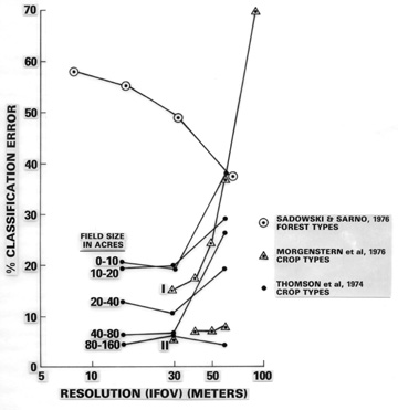
The dramatic improvement in reducing errors around 30 m (98 ft) relates, in part, to the nature of the target classes. Coarse resolution is ineffective in distinguishing crop types, but high resolution (< 20 m) adds little in recognizing these other than perhaps identifying species. As the size of crop fields increases, the error decreases further. The anomalous trend for forests (maximum error at high resolution) may be the consequence of the dictum: “Can’t see the forest for the trees. Here, this saying means that high resolution begins to display individual species and breaks in the canopy that can confuse the integrity of the class “forest”. Two opposing trends influence the behavior of these error curves: 1) statistical variance of the spectral response values decreases whereas 2) the proportion of mixed pixels increases with lower resolution.
A study of classification accuracy as a function of the number of spectral bands shows these trends:
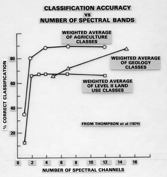
The increase from one to two bands produces the largest improvement in accuracy. After about four bands, the accuracy increase flattens or increases very slowly. Thus, extra bands may be redundant, because band-to-band changes cross-correlate (this correlation may be minimized and even put to advantage through Principal Components Analysis). However, additional bands, such as TM bands 5 and 7, can be helpful in identifying rock types (geology), because various rock types absorb certain wavelengths, which helps identify them in these spectral intervals. Note that the highest accuracy associates with crop types because fields, consisting of regularly-space rows of plants against a background of soil, tend to be more uniform .
In practice, we may test classification accuracy in four ways: 1) field checks at selected points (usually non-rigorous and subjective), chosen either at random or along a grid; 2) estimate (non-rigorous) the agreement of the theme or class identity between a class map and reference maps, determined usually by overlaying one on the other(s); 3) statistical analysis (rigorous) of numerical data developed in sampling, measuring, and processing data, using tests, such as root mean square, standard error, analysis of variance, correlation coefficients, linear or multiple regression analysis, and Chi-square testing (see any standard text on statistics for an explanation of these tests); and 4) confusion matrix calculations (rigorous). We explain this last approach using the author’s study of a subscene from a July, 1977, Landsat image that includes Elkton, Maryland (top center).
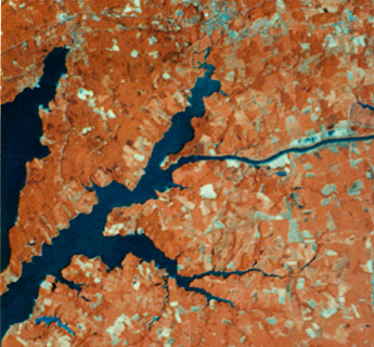
We acquired a 1:24,000 aerial photo that falls within this subscene from the EPA. Starting with a field visit in August, 1977, during the same growing season as the July overflight, we identified the crops in many farms located in the photo, of which we selected about 12 as training sites. Most were either corn or soybeans, and others were mainly barley and wheat. We then ran a Maximum Likelihood supervised classification, as shown below, and printed as a transparency.
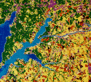

We overlaid this transparency onto a rescaled aerial photo until field patterns approximately matched. With the class identities in the photo as the standard, we arranged the number of pixels correctly assigned to each class and those misassigned to other classes in the confusion matrix used to produce the summary information shown in Table 13-2, listing errors of commission, omission, and overall accuracies. Errors of commission result when we incorrectly identify pixels associated with a class as other classes, or when we improperly separate a single class into two or more classes. Errors of omission occur whenever we simply don’t recognize pixels that we should have identified as belonging to a particular class.

` <>`__13-7: Why are the mapping accuracies for individual classes lower than that of the overall classification? `ANSWER <Sect13_answers.html#13-7>`__
` <>`__13-8: Discuss and explain what is meant by errors of commision and omission for corn. `ANSWER <Sect13_answers.html#13-8>`__
` <>`__13-9: List at least five scene-dependent sources of error for the above case. `ANSWER <Sect13_answers.html#13-9>`__
Mapping accuracy for each class is the number of correctly identified pixels within the displayed area, divided by that number plus error pixels of commission and omission. To illustrate, in the table, of the 43 pixels classed as corn by photointerpretation and ground checks, we assigned 25 of these to corn in the Landsat classification, leaving 18/43 = 42% as the error of omission. Similarly, of the 43, we improperly identified 7 as other than corn, producing a commission error of 16%. After we determine these errors by reference to “ground truth”, we can reduce them by selecting new training sites and reclassifying them, by renaming classes or creating new ones, by combining them, or by using different classifiers. With each set of changes, we iterate the classification procedure until we reach a final level of acceptable accuracy.
Primary Author: Nicholas M. Short, Sr. email: nmshort@nationi.net